Tutorial on tensorflow usage

Outline

• Brief introduction to tensorflow
• Start from a simple CNN
• Utilities
• Advanced API
• Dynamic mode
• Appendixes

1. Brief introduction to tensorflow

1.1. Architectures of CPU and GPU

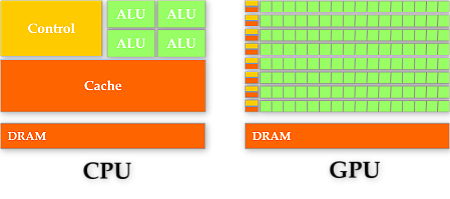
• CPU: master in cache and flow control
• GPU: master in numerical calculation

1.2. Tensorflow architecture

1.2.1. The programming stack

• An open-source software library
• Run on multiple (distri) CPUs and GPUs (TPUs)
• Support Python, C++, JAVA, Go

1.2.2. Units

• Perform computing tasks as a graph
• Execute the graph in the context of session
• Represent data as tensor
• Maintaining states through variable
• Use feed and fetch to assign values to arbitrary operation or obtain values from it

import tensorflow as tf
# Creat a variable and initialize it as scalar 0
state = tf.Variable(0, name="counter")
# To creat an op, aiming to increase state by 1
one = tf.placeholder(tf.int32, shape=None, name='one')
new_value = tf.add(state, one)
update = tf.assign(state, new_value)
# After the graph startup, variables must be initialized
# First, add an `initializer` op into the graph
init_op = tf.global_variables_initializer()
# Start the graph, run ops
with tf.Session() as sess:
  # Run 'init' op
  sess.run(init_op)
  # Print the initial value of 'state'
  print(sess.run(state))
  # Run op to update 'state' and print 'state'
  for _ in range(3):
    sess.run(update, feed_dict={one:1})
    print(sess.run(state))
# Output:
# 0
# 1
# 2
# 3

1.2.3. GPU usage

• Visual studio (2015)
• python 2.7 or 3.5+
• CUDA and cuDNN
• pip or whl tensorflow-gpu

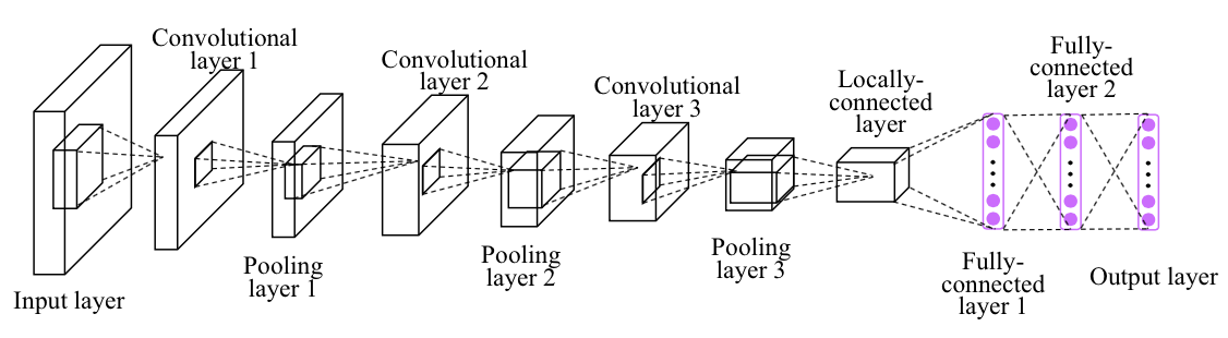
2. Start from a simple CNN

2.1. Convolutional neural network model

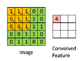
2.1.1. Convolution

• convolutional kernel
• stride
• padding
  

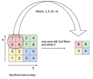
2.1.2. Pooling

• max pooling
• mean pooling

2.2. MNIST database

• 60,000 examples for training and 10,000 examples for testing
• size-normalized and centered in a fixed-size image (28x28 pixels)
• flattened and converted to a 1-D numpy array of 784 features

tensorflow.examples.tutorials.mnist

2.3. Code implementation

2.3.1. Preliminary

from __future__ import division, print_function, absolute_import
import tensorflow as tf
# Import MNIST data
from tensorflow.examples.tutorials.mnist import input_data
mnist = input_data.read_data_sets("/tmp/data/", one_hot=True)
# Training Parameters
learning_rate = 0.001
num_steps = 500
batch_size = 128
display_step = 10
# Network Parameters
num_input = 784 # MNIST data input (img shape: 28*28)
num_classes = 10 # MNIST total classes (0-9 digits)
dropout = 0.75 # Dropout, probability to keep units
# tf Graph input
X = tf.placeholder(tf.float32, [None, num_input])
Y = tf.placeholder(tf.float32, [None, num_classes])
keep_prob = tf.placeholder(tf.float32) # dropout (keep probability)

2.3.2. Creat model architecture

# Create some wrappers for simplicity
def conv2d(x, W, b, strides=1):
    # Conv2D wrapper, with bias and relu activation
    x = tf.nn.conv2d(x, W, strides=[1, strides, strides, 1], padding='SAME')
    x = tf.nn.bias_add(x, b)
    return tf.nn.relu(x)
def maxpool2d(x, k=2):
    # MaxPool2D wrapper
    return tf.nn.max_pool(x, ksize=[1, k, k, 1], strides=[1, k, k, 1],
                          padding='SAME')
# Create model
def conv_net(x, weights, biases, dropout):
    # MNIST data input is a 1-D vector of 784 features (28*28 pixels)
    # Reshape to match picture format [Height x Width x Channel]
    # Tensor input become 4-D: [Batch Size, Height, Width, Channel]
    x = tf.reshape(x, shape=[-1, 28, 28, 1])
    # Convolution Layer
    conv1 = conv2d(x, weights['wc1'], biases['bc1'])
    # Max Pooling (down-sampling)
    conv1 = maxpool2d(conv1, k=2)
    # Convolution Layer
    conv2 = conv2d(conv1, weights['wc2'], biases['bc2'])
    # Max Pooling (down-sampling)
    conv2 = maxpool2d(conv2, k=2)
    # Fully connected layer
    # Reshape conv2 output to fit fully connected layer input
    fc1 = tf.reshape(conv2, [-1, weights['wd1'].get_shape().as_list()[0]])
    fc1 = tf.add(tf.matmul(fc1, weights['wd1']), biases['bd1'])
    fc1 = tf.nn.relu(fc1)
    # Apply Dropout
    fc1 = tf.nn.dropout(fc1, dropout)
    # Output, class prediction
    out = tf.add(tf.matmul(fc1, weights['out']), biases['out'])
    return out

2.3.3. Construct model graph

# Store layers weight & bias
weights = {
    # 5x5 conv, 1 input, 32 outputs
    'wc1': tf.Variable(tf.random_normal([5, 5, 1, 32])),
    # 5x5 conv, 32 inputs, 64 outputs
    'wc2': tf.Variable(tf.random_normal([5, 5, 32, 64])),
    # fully connected, 7*7*64 inputs, 1024 outputs
    'wd1': tf.Variable(tf.random_normal([7*7*64, 1024])),
    # 1024 inputs, 10 outputs (class prediction)
    'out': tf.Variable(tf.random_normal([1024, num_classes]))
}
biases = {
    'bc1': tf.Variable(tf.random_normal([32])),
    'bc2': tf.Variable(tf.random_normal([64])),
    'bd1': tf.Variable(tf.random_normal([1024])),
    'out': tf.Variable(tf.random_normal([num_classes]))
}
# Construct model
logits = conv_net(X, weights, biases, keep_prob)
prediction = tf.nn.softmax(logits)
# Define loss and optimizer
loss_op = tf.reduce_mean(tf.nn.softmax_cross_entropy_with_logits(
    logits=logits, labels=Y))
optimizer = tf.train.AdamOptimizer(learning_rate=learning_rate)
train_op = optimizer.minimize(loss_op)
# Evaluate model
correct_pred = tf.equal(tf.argmax(prediction, 1), tf.argmax(Y, 1))
accuracy = tf.reduce_mean(tf.cast(correct_pred, tf.float32))
# Initialize the variables (i.e. assign their default value)
init = tf.global_variables_initializer()

2.3.4. Session run

# Start training
with tf.Session() as sess:
    # Run the initializer
    sess.run(init)
    for step in range(1, num_steps+1):
        batch_x, batch_y = mnist.train.next_batch(batch_size)
        # Run optimization op (backprop)
        sess.run(train_op, feed_dict={X: batch_x, Y: batch_y, keep_prob: dropout})
        if step % display_step == 0 or step == 1:
            # Calculate batch loss and accuracy
            loss, acc = sess.run([loss_op, accuracy], feed_dict={X: batch_x,
                                                                 Y: batch_y,
                                                                 keep_prob: 1.0})
            print("Step " + str(step) + ", Minibatch Loss= " + \
                  "{:.4f}".format(loss) + ", Training Accuracy= " + \
                  "{:.3f}".format(acc))
    print("Optimization Finished!")
    # Calculate accuracy for 256 MNIST test images
    print("Testing Accuracy:", \
        sess.run(accuracy, feed_dict={X: mnist.test.images[:256],
                                      Y: mnist.test.labels[:256],
                                      keep_prob: 1.0}))
# Testing Accuracy: 0.976562

3. Utilities

3.1. Save and restore model

# 'Saver' op to save and restore all the variables
saver = tf.train.Saver()
# Save model weights to disk
save_path = saver.save(sess, model_path)
print("Model saved in file: %s" % save_path)
 # Restore model weights from previously saved model
load_path = saver.restore(sess, model_path)
print("Model restored from file: %s" % save_path)

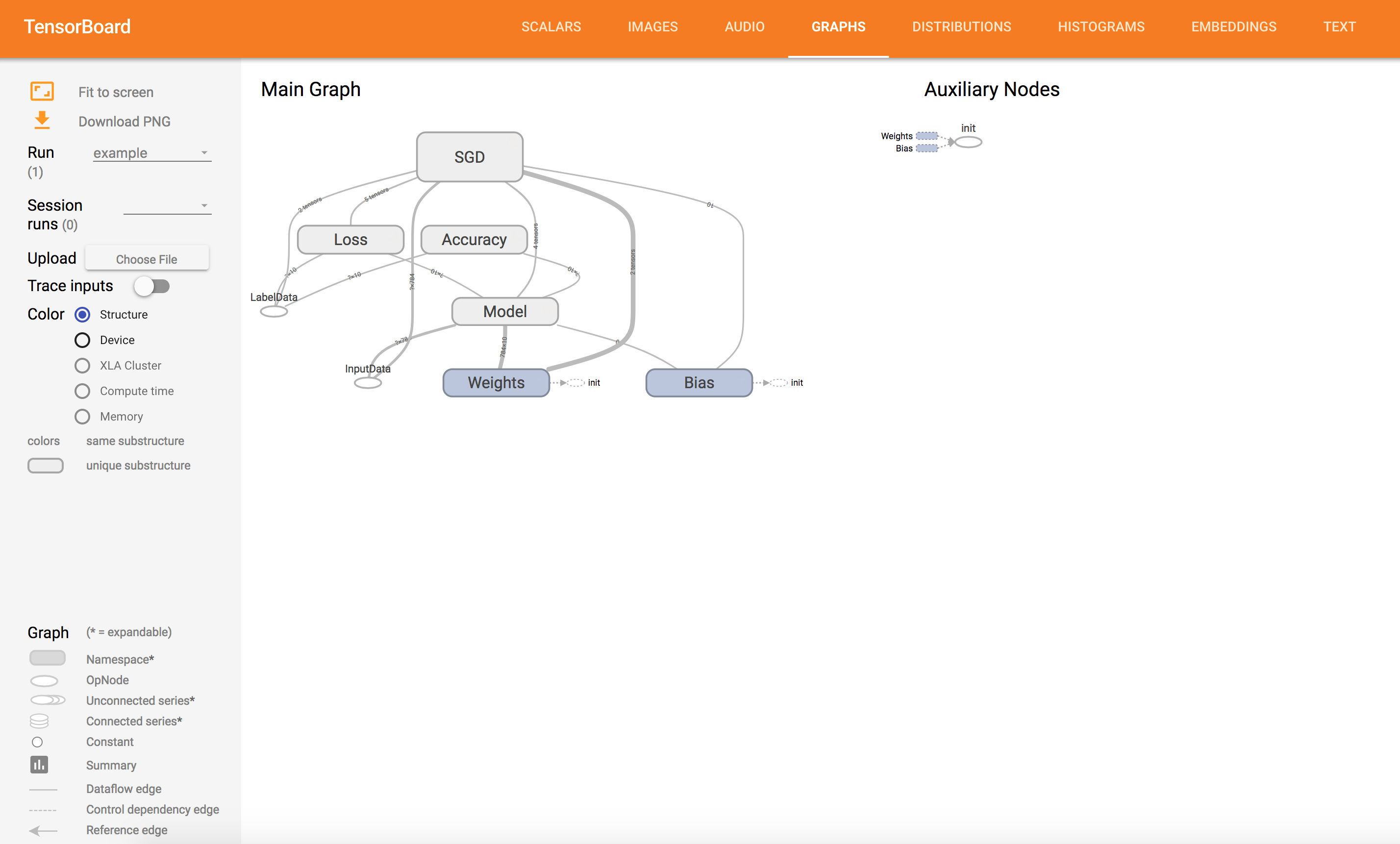
3.2. Visualization - tensorboard basics

# Construct model and encapsulating all ops into scopes, making
# Tensorboard's Graph visualization more convenient
with tf.name_scope('Model'):
    # Model
    pred = tf.nn.softmax(tf.matmul(x, W) + b) # Softmax
with tf.name_scope('Loss'):
    # Minimize error using cross entropy
    cost = tf.reduce_mean(-tf.reduce_sum(y * tf.log(pred), reduction_indices=1))
with tf.name_scope('SGD'):
    # Gradient Descent
    optimizer = tf.train.GradientDescentOptimizer(learning_rate).minimize(cost)
with tf.name_scope('Accuracy'):
    # Accuracy
    acc = tf.equal(tf.argmax(pred, 1), tf.argmax(y, 1))
    acc = tf.reduce_mean(tf.cast(acc, tf.float32))
# Initializing the variables
init = tf.global_variables_initializer()
# Create a summary to monitor cost tensor
tf.summary.scalar("loss", cost)
# Create a summary to monitor accuracy tensor
tf.summary.scalar("accuracy", acc)
# Merge all summaries into a single op
merged_summary_op = tf.summary.merge_all()
# Start Training
with tf.Session() as sess:
    sess.run(init)
    # op to write logs to Tensorboard
    summary_writer = tf.summary.FileWriter(logs_path, graph=tf.get_default_graph())
    # ...
        # Run optimization op (backprop), cost op (to get loss value)
        # and summary nodes
        _, c, summary = sess.run([optimizer, cost, merged_summary_op],
                                feed_dict={x: batch_xs, y: batch_ys})
        # Write logs at every iteration
        summary_writer.add_summary(summary, epoch * total_batch + i)
# Run the command line:
# --> tensorboard --logdir=/tmp/tensorflow_logs 
# Then open http://0.0.0.0:6006/ into your web browser

Loss and Accuracy Visualization

Graph Visualization

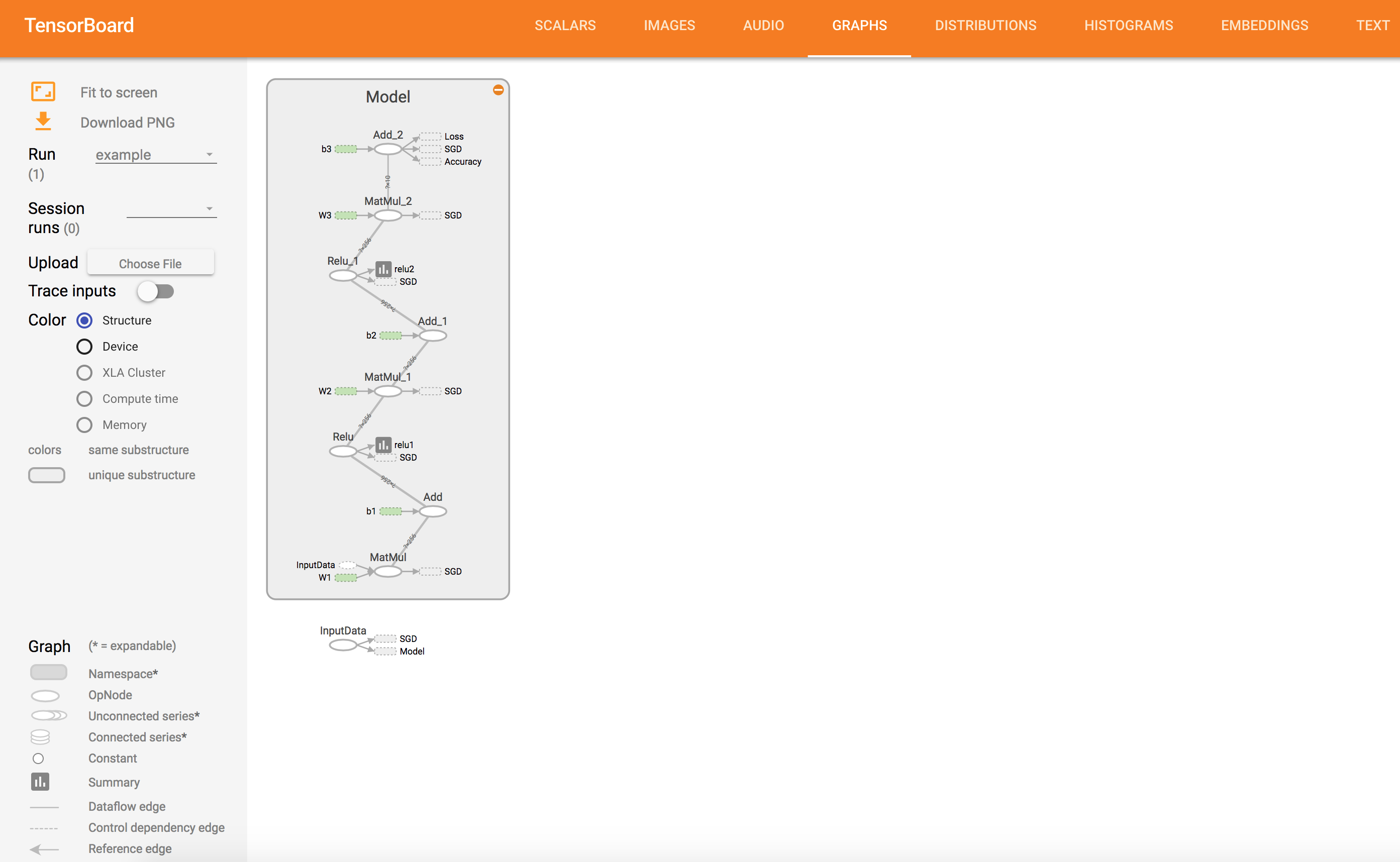
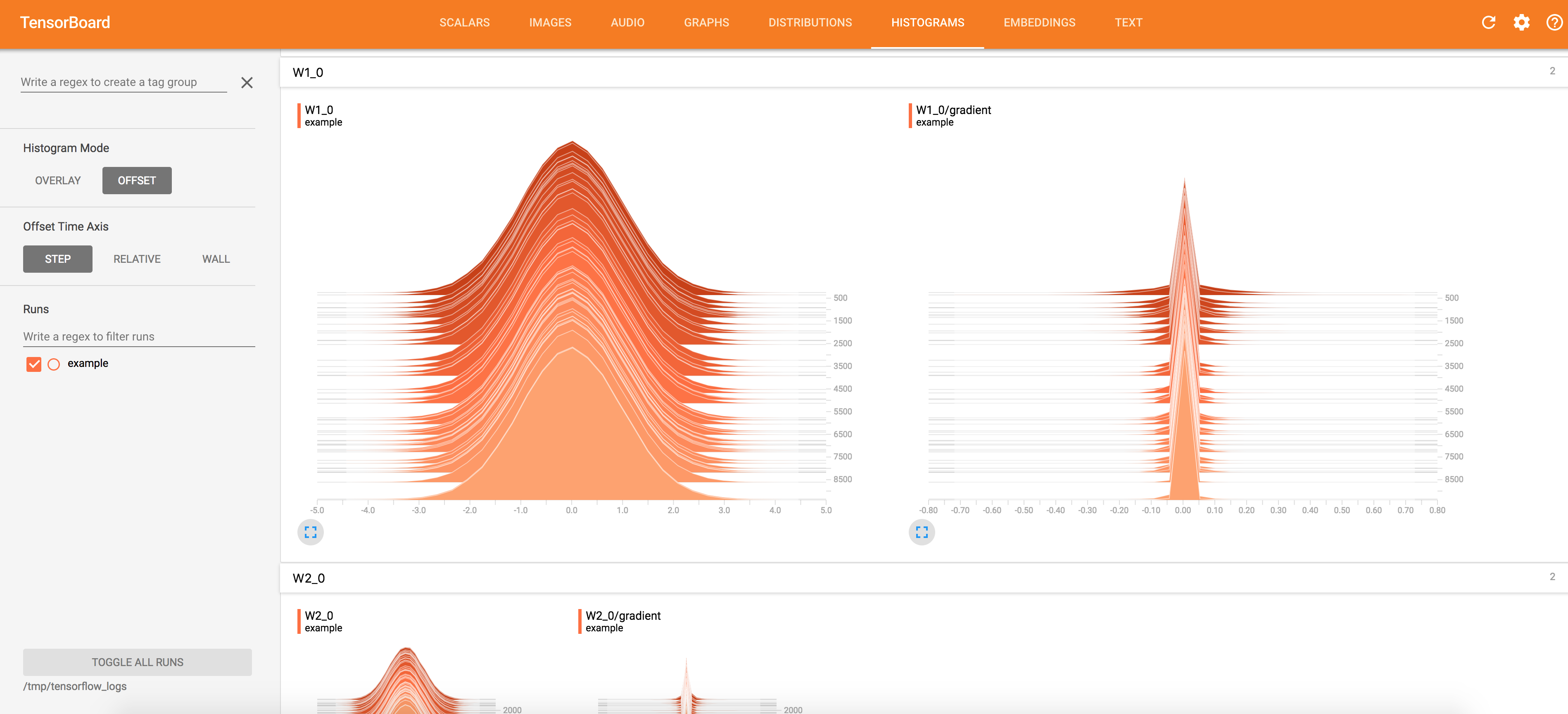
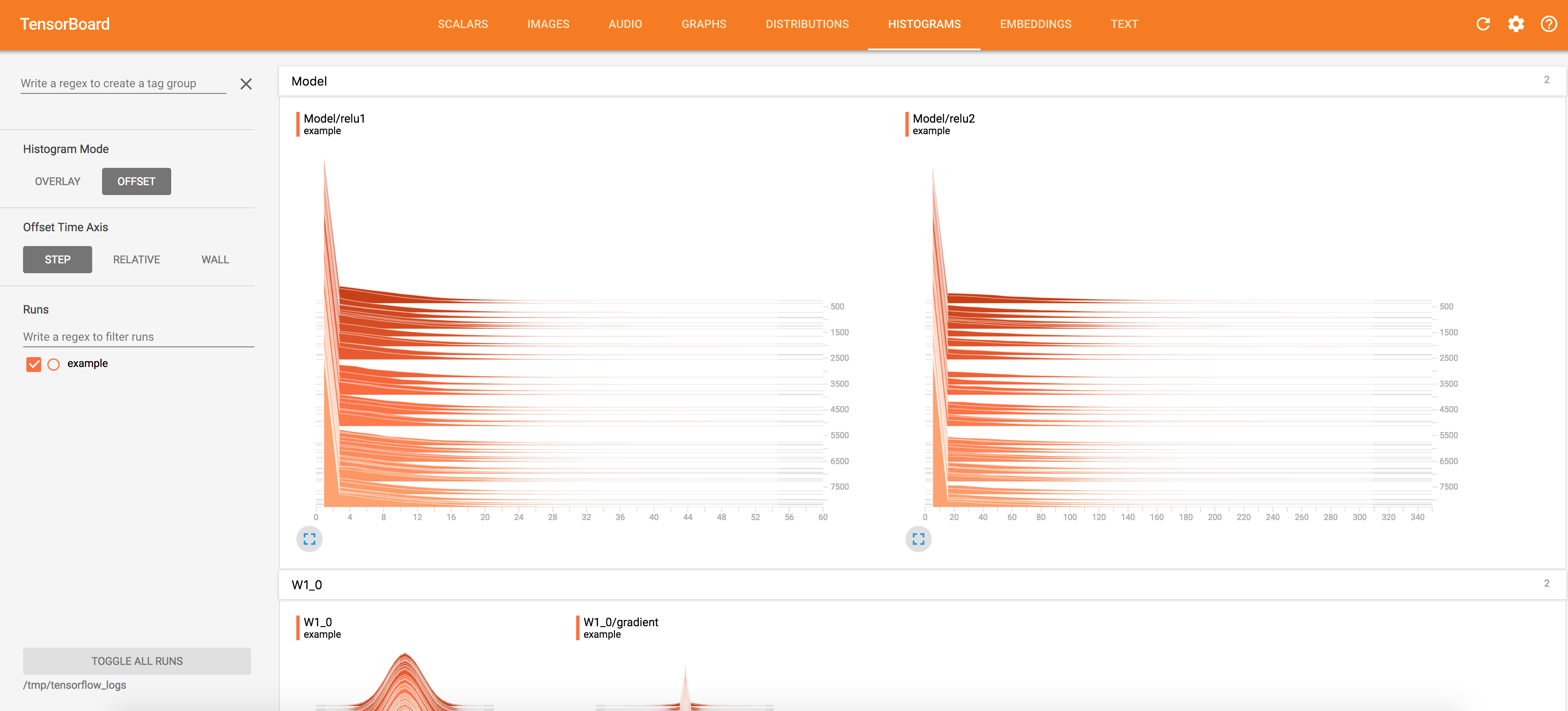
3.3. Visualization - tensorboard advanced

with tf.name_scope('SGD'):
    # Gradient Descent
    optimizer = tf.train.GradientDescentOptimizer(learning_rate)
    # Op to calculate every variable gradient
    grads = tf.gradients(loss, tf.trainable_variables())
    grads = list(zip(grads, tf.trainable_variables()))
    # Op to update all variables according to their gradient
    apply_grads = optimizer.apply_gradients(grads_and_vars=grads)
# Create summaries to visualize weights
for var in tf.trainable_variables():
    tf.summary.histogram(var.name, var)
# Summarize all gradients
for grad, var in grads:
    tf.summary.histogram(var.name + '/gradient', grad)

Computation Graph Visualization

Weights and Gradients Visualization

Activations Visualization

4. Advanced APIs

4.1. High-level package

4.1.1. Keras

from tensorflow import keras

# Sequential model
model = keras.Sequential()
# Adds a densely-connected layer with 64 units to the model:
model.add(keras.layers.Dense(64, activation='relu'))
# Add another:
model.add(keras.layers.Dense(64, activation='relu'))
# Add a softmax layer with 10 output units:
model.add(keras.layers.Dense(10, activation='softmax'))

# Set up training
model.compile(optimizer=tf.train.AdamOptimizer(0.001),
              loss='categorical_crossentropy',
              metrics=['accuracy'])
# Input NumPy data
model.fit(data, labels, epochs=10, batch_size=32)
# Evaluate and predict
model.evaluate(x, y, batch_size=32)
model.predict(x, batch_size=32)

from keras.applications import inception_v3

4.1.2. Slim (Tensorlayer)

import tensorflow.contrib.slim as slim

with slim.arg_scope([slim.conv2d], padding='SAME',
                    weights_initializer=tf.truncated_normal_initializer(stddev=0.01)
                    weights_regularizer=slim.l2_regularizer(0.0005)):
    net = slim.conv2d(inputs, 64, [11, 11], scope='conv1')
    net = slim.conv2d(net, 128, [11, 11], padding='VALID', scope='conv2')
    net = slim.conv2d(net, 256, [11, 11], scope='conv3')

net = ...
net = slim.conv2d(net, 256, [3, 3], scope='conv3_1')
net = slim.conv2d(net, 256, [3, 3], scope='conv3_2')
net = slim.conv2d(net, 256, [3, 3], scope='conv3_3')
net = slim.max_pool2d(net, [2, 2], scope='pool2')
# using slim.repeat
net = slim.repeat(net, 3, slim.conv2d, 256, [3, 3], scope='conv3')
net = slim.max_pool2d(net, [2, 2], scope='pool2')

x = slim.fully_connected(x, 32, scope='fc/fc_1')
x = slim.fully_connected(x, 64, scope='fc/fc_2')
x = slim.fully_connected(x, 128, scope='fc/fc_3')
# using slim.stack
slim.stack(x, slim.fully_connected, [32, 64, 128], scope='fc')

4.2. Estimator

# Define the input function for training
input_fn = tf.estimator.inputs.numpy_input_fn(
    x={'images': mnist.train.images}, y=mnist.train.labels,
    batch_size=batch_size, num_epochs=None, shuffle=True)

# Define the neural network
def neural_net(x_dict):
    # TF Estimator input is a dict, in case of multiple inputs
    x = x_dict['images']
    # Hidden fully connected layer with 256 neurons
    layer_1 = tf.layers.dense(x, n_hidden_1)
    # Hidden fully connected layer with 256 neurons
    layer_2 = tf.layers.dense(layer_1, n_hidden_2)
    # Output fully connected layer with a neuron for each class
    out_layer = tf.layers.dense(layer_2, num_classes)
    return out_layer

# Define the model function (following TF Estimator Template)
def model_fn(features, labels, mode):
    # Build the neural network
    logits = neural_net(features)
    # Predictions
    pred_classes = tf.argmax(logits, axis=1)
    pred_probas = tf.nn.softmax(logits)
    # If prediction mode, early return
    if mode == tf.estimator.ModeKeys.PREDICT:
        return tf.estimator.EstimatorSpec(mode, predictions=pred_classes) 
    # Define loss and optimizer
    loss_op = tf.reduce_mean(tf.nn.sparse_softmax_cross_entropy_with_logits(
        logits=logits, labels=tf.cast(labels, dtype=tf.int32)))
    optimizer = tf.train.GradientDescentOptimizer(learning_rate=learning_rate)
    train_op = optimizer.minimize(loss_op, global_step=tf.train.get_global_step())
    # Evaluate the accuracy of the model
    acc_op = tf.metrics.accuracy(labels=labels, predictions=pred_classes)
    # TF Estimators requires to return a EstimatorSpec, that specify
    # the different ops for training, evaluating, ...
    estim_specs = tf.estimator.EstimatorSpec(
      mode=mode,
      predictions=pred_classes,
      loss=loss_op,
      train_op=train_op,
      eval_metric_ops={'accuracy': acc_op})
    return estim_specs

# Build the Estimator
model = tf.estimator.Estimator(model_fn)
# Train the Model
model.train(input_fn, steps=num_steps)

Checkpoint

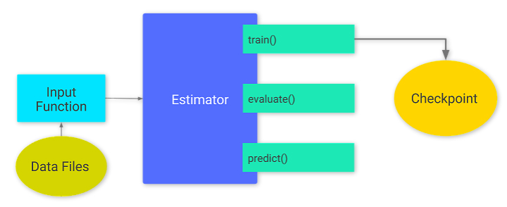
• Estimators automatically write the following to disk:
  
  • checkpoints, which are versions of the model created during training.
  • event files, which contain information that TensorBoard uses to create visualizations.

my_checkpointing_config = tf.estimator.RunConfig(
    save_checkpoints_secs = 20*60,  # Save checkpoints every 20 minutes.
    keep_checkpoint_max = 10,       # Retain the 10 most recent checkpoints.
)
classifier = tf.estimator.DNNClassifier(
    feature_columns=my_feature_columns,
    hidden_units=[10, 10],
    n_classes=3,
    model_dir='models/iris',
    config=my_checkpointing_config)

4.3. Dataset

# Create a dataset tensor from the images and the labels
dataset = tf.contrib.data.Dataset.from_tensor_slices(
    (mnist.train.images, mnist.train.labels))
# Create batches of data
dataset = dataset.batch(batch_size)
# Create an iterator, to go over the dataset
iterator = dataset.make_initializable_iterator()
# It is better to use 2 placeholders, to avoid to load all data into memory,
# and avoid the 2Gb restriction length of a tensor.
_data = tf.placeholder(tf.float32, [None, n_input])
_labels = tf.placeholder(tf.float32, [None, n_classes])
# Initialize the iterator
sess.run(iterator.initializer, feed_dict={_data: mnist.train.images,
                                          _labels: mnist.train.labels})
# Neural Net Input
X, Y = iterator.get_next()

5. Dynamic mode

5.1. Dynamic graph

• Static declaration VS Dynamic declaration
• Declaration & Execution
• Virtual computing graph & Entity computing graph
• Layout, memory allocation, execution: Global VS Local
• Efficiency VS Friendly coding
• Multi-structure input problem
  
  • TensorFlow Fold via Dynamic Batching
  • Simulate dynamic graphs with arbitrary shape and size
  • https://zhuanlan.zhihu.com/p/25216368
• (Pytorch is also quite popular in academic researches)

5.2. Eager mode

Eager API basics

# Set Eager API
tf.enable_eager_execution()
tfe = tf.contrib.eager
# Run the operation without the need for tf.Session
a = tf.constant(2)
b = tf.constant(3)
c = a + b
d = a * b
# Full compatibility with Numpy
a = tf.constant([[2., 1.],
                 [1., 0.]], dtype=tf.float32)
b = np.array([[3., 0.],
              [5., 1.]], dtype=np.float32)
c = a + b
d = tf.matmul(a, b)
# Auto differentiation
def square(x):
  return tf.multiply(x, x)
grad = tfe.gradients_function(square)
square(3.)  # => 9.0
grad(3.)    # => [6.0]

A toy example

class Model(tf.keras.Model):
  def __init__(self):
    super(Model, self).__init__()
    self.W = tfe.Variable(5., name='weight')
    self.B = tfe.Variable(10., name='bias')
  def call(self, inputs):
    return inputs * self.W + self.B
# A toy dataset of points around 3 * x + 2
NUM_EXAMPLES = 2000
training_inputs = tf.random_normal([NUM_EXAMPLES])
noise = tf.random_normal([NUM_EXAMPLES])
training_outputs = training_inputs * 3 + 2 + noise
# The loss function to be optimized
def loss(model, inputs, targets):
  error = model(inputs) - targets
  return tf.reduce_mean(tf.square(error))
def grad(model, inputs, targets):
  with tf.GradientTape() as tape:
    loss_value = loss(model, inputs, targets)
  return tape.gradient(loss_value, [model.W, model.B])
# Define:
# 1. A model.
# 2. Derivatives of a loss function with respect to model parameters.
# 3. A strategy for updating the variables based on the derivatives.
model = Model()
optimizer = tf.train.GradientDescentOptimizer(learning_rate=0.01)
print("Initial loss: {:.3f}".format(loss(model, training_inputs, training_outputs)))
# Training loop
for i in range(300):
  grads = grad(model, training_inputs, training_outputs)
  optimizer.apply_gradients(zip(grads, [model.W, model.B]),
                            global_step=tf.train.get_or_create_global_step())
  if i % 20 == 0:
    print("Loss at step {:03d}: {:.3f}".format(i, loss(model, training_inputs, training_outputs)))
print("Final loss: {:.3f}".format(loss(model, training_inputs, training_outputs)))
print("W = {}, B = {}".format(model.W.numpy(), model.B.numpy()))

Save and restore in eager mode

model = MyModel()
optimizer = tf.train.AdamOptimizer(learning_rate=0.001)
checkpoint_dir = ‘/path/to/model_dir’
checkpoint_prefix = os.path.join(checkpoint_dir, "ckpt")
root = tfe.Checkpoint(optimizer=optimizer,
                      model=model,
                      optimizer_step=tf.train.get_or_create_global_step())
root.save(file_prefix=checkpoint_prefix)
# or
root.restore(tf.train.latest_checkpoint(checkpoint_dir))

Tensorboard in eager mode

writer = tf.contrib.summary.create_file_writer(logdir)
global_step=tf.train.get_or_create_global_step()  # return global step var
writer.set_as_default()
for _ in range(iterations):
  global_step.assign_add(1)
  # Must include a record_summaries method
  with tf.contrib.summary.record_summaries_every_n_global_steps(100):
    # your model code goes here
    tf.contrib.summary.scalar('loss', loss)
     ...

Use eager execution in a graph environment

def my_py_func(x):
  x = tf.matmul(x, x)  # You can use tf ops
  print(x)  # but it's eager!
  return x
with tf.Session() as sess:
  x = tf.placeholder(dtype=tf.float32)
  # Call eager function in graph!
  pf = tfe.py_func(my_py_func, [x], tf.float32)
  sess.run(pf, feed_dict={x: [[2.0]]})  # [[4.0]]

5.3. AutoGraph (beta)

pip install -U tf-nightly

from tensorflow.contrib import autograph as ag

Using with annotations

@ag.convert()
def f(x):
  if x < 0:
    x = -x
  return x

with tf.Graph().as_default():
  x = tf.constant(-1)
  y = f(x)
  with tf.Session() as sess:
    print(sess.run(y))
    # Output: 1

Using the functional API

converted_f = ag.to_graph(f)
print(converted_f(tf.constant(-1)))
# Output: Tensor
print(f(-1))
# Output: 1

print(ag.to_code(f))
# Output: <Python and TensorFlow code>

6. Appendixs

6.1. Tricks

Learning rate decay

  global_step = tf.Variable(0, trainable=False)
  starter_learning_rate = 0.1
  learning_rate = tf.train.exponential_decay(starter_learning_rate, global_step,
                                             100000, 0.96)
  # Passing global_step to minimize() will increment it at each step.
  learning_step = (
      tf.train.GradientDescentOptimizer(learning_rate)
      .minimize(...my loss..., global_step=global_step)
  )

decayed_learning_rate = learning_rate *
                          decay_rate ^ (global_step / decay_steps)

Find anywhere 'nan' is raised

check= tf.add_check_numerics_ops
...
sess.run([check, ...])

Filter which layer to be freezed through variable names

tvars = tf.trainable_variables()
tvars = [v for v in tvars if 'frozen' not in v.name]
grads = tf.gradients(loss, tvars)

Leverage Timeline to analyse time consumption

run_metadata = tf.RunMetadata()
run_options = tf.RunOptions(trace_level=tf.RunOptions.FULL_TRACE)
config = tf.ConfigProto(graph_options=tf.GraphOptions(
        optimizer_options=tf.OptimizerOptions(opt_level=tf.OptimizerOptions.L0)))
with tf.Session(config=config) as sess:
    c_np = sess.run(c,options=run_options,run_metadata=run_metadata)
    tl = timeline.Timeline(run_metadata.step_stats)
    ctf = tl.generate_chrome_trace_format()
with open('timeline.json','w') as wd:
    wd.write(ctf)
# Open chrome and type: chrome://tracing
# and import timeline.json

......

6.2. Extended libraries

Cupy, Dask

# 在一个cpu上跑 
import numpy as np
x = np.random.random((2,3))  
y = x.T.dot(np.log(x) + 1)
z = y - y.mean(axis=0)
print(z[:5])
# 在GPU上跑
import cupy as cp
x = cp.random.random((2,3))  
y = x.T.dot(cp.log(x) + 1)
z = y - y.mean()
print(z[:5].get())
# 在许多cpu上跑
import dask.array as da
x = da.random.random((2,3))  
y = x.T.dot(da.log(x) + 1)
z = y - y.mean(axis=0)
print(z[:5].compute())

Ray (under development)

• Ray is a Python-based distributed execution engine.
• Developed by RISELab (AMPLab as the predecessor).
• The same code can be run on a single machine to achieve efficient multiprocessing,
  and it can be used on a cluster for large computations.
• Asynchronous parallel.
• scheduling latency:
  
  • 100us level (Ray) vs 100ms level (Spark)
• dynamic tasks

def add1(a, b):
    return a + b
@ray.remote
def add2(a, b):
    return a + b
x_id = add2.remote(1, 2)
ray.get(x_id)  # 3

import time
def f1():
    time.sleep(1)
@ray.remote
def f2():
    time.sleep(1)
# The following takes ten seconds.
[f1() for _ in range(10)]
# The following takes one second (assuming the system has at least ten CPUs).
ray.get([f2.remote() for _ in range(10)])

@ray.remote
def f(x):
    return x + 1
x = f.remote(0)
y = f.remote(x)
z = f.remote(y)
ray.get(z) # 3

TensorLy

......

Suggestion

Tensorflow + Slim (TensorLayer)
Estimator + Checkpoint + TensorBoard
Eager execution if you want