@SmashStack
2017-05-03T18:10:48.000000Z
字数 34292
阅读 3946
无线网络攻防实验平台实验报告
Chore
实验人员: 张 倬
报告作者: 张 倬
学 号: 5140369057
完成时间: 2017 年 5 月 3 日
NS2 安装与配置
一、实验目的
- 掌握 Linux 环境下 NS2 软件的安装工作;
- 熟悉 NS2 环境变量的设置。
二、实验内容
1. Linux 上 NS2 必要工具和库文件的安装;
2. Linux 上 NS2 软件的安装;
3. NS2 环境变量的设置;
4. 安装结果的验证。
三、实验步骤及测试结果
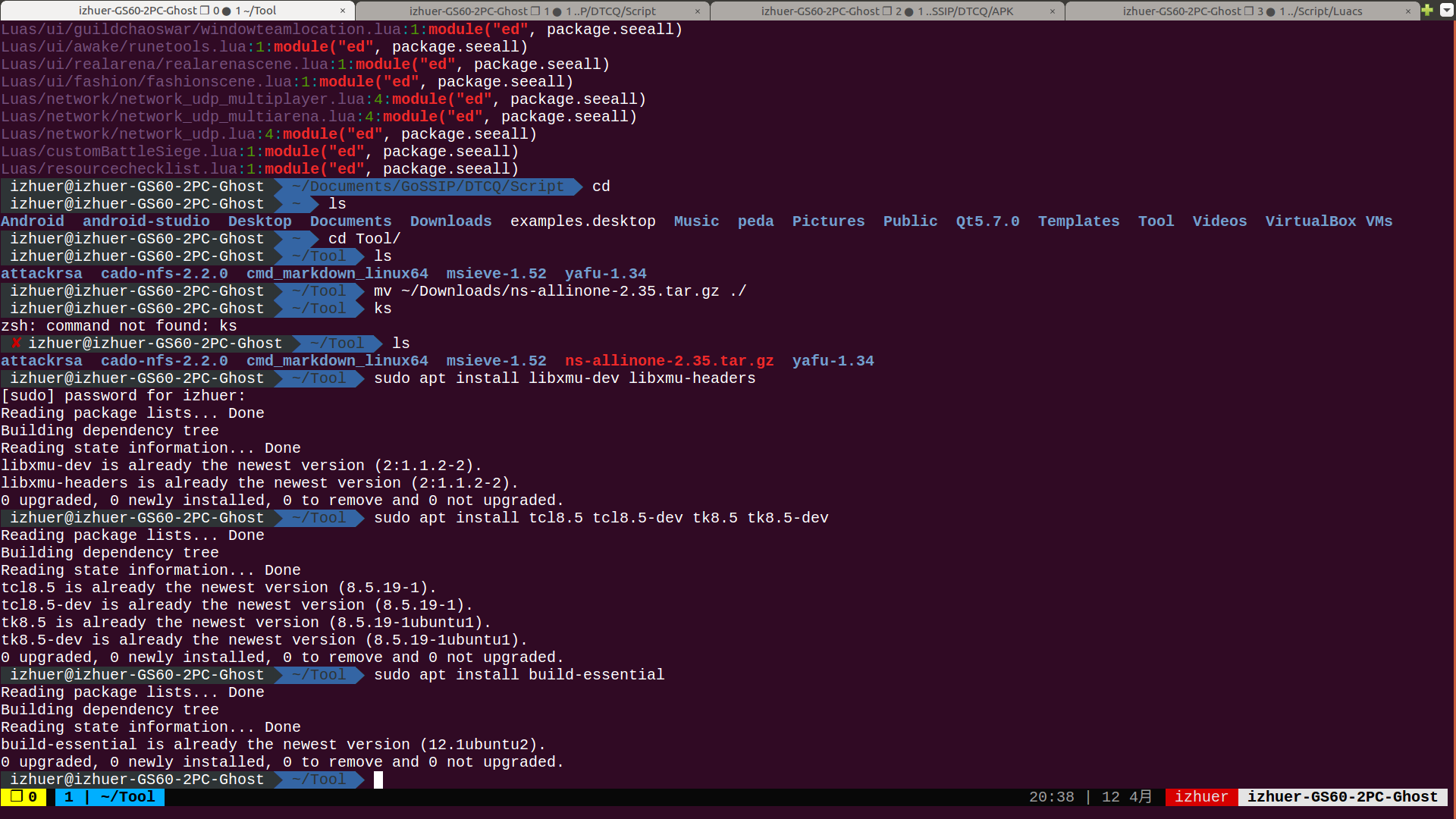
- NS2 必要工具和库文件的安装
- sudo apt install build-essential
- sudo apt install tcl8.5 tcl8.5-dev tk8.5 tk8.5-dev
- sudo apt install libxmu-dev libxmu-headers
- NS2 的安装
- 在 http://sourceforge.net/projects/nsnam/files/ns-2/2.35/ns-src-2.35.tar.gz/download 上下载 NS2 的安装压缩包 ns2-allinone-2.35.tar.gz,放在安装路径的目录文件夹下
- 进入该目录,并解压 ns2-allinone-2.35.tar.gz 包到当前目录
- 进入解压后的文件夹,开始安装
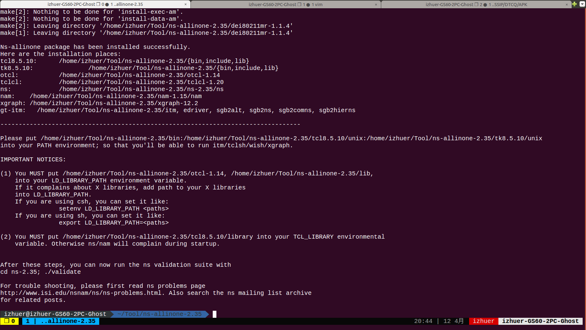
- 设置环境变量
- 打开~/.zshrc文件进行编辑,如下图所示(我 Ubuntu 使用的是 zsh,所以修改 .zshrc 文件):

- 打开~/.zshrc文件进行编辑,如下图所示(我 Ubuntu 使用的是 zsh,所以修改 .zshrc 文件):
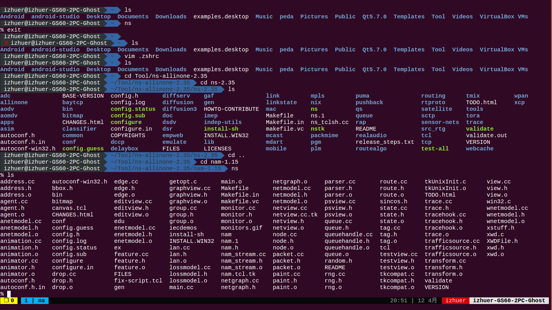
- 验证环境变量配置是否正确
- ns2安装成功
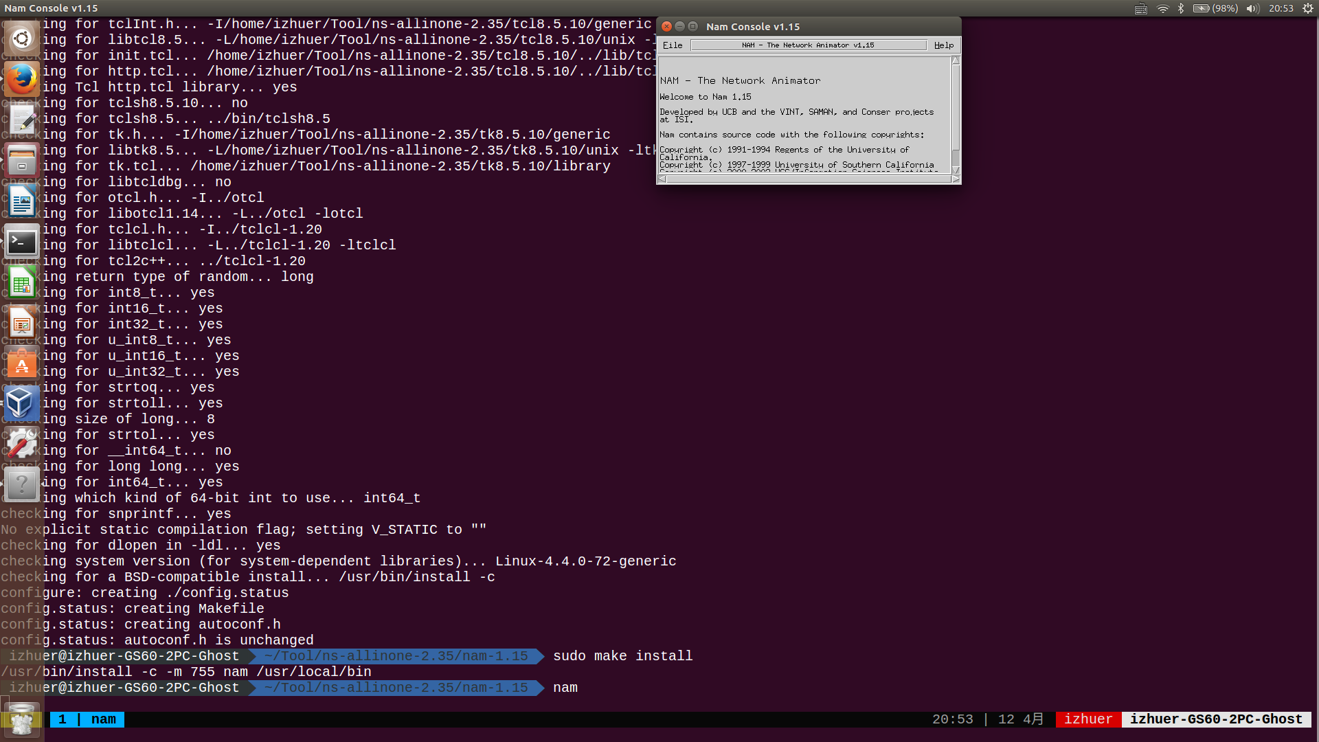
- nam安装成功
- ns2安装成功
四、实验心得与体会
这次实验特别锻炼了我独立解决问题的能力,在编译 ns2 的过程中,我曾经遇到了如下的报错信息:
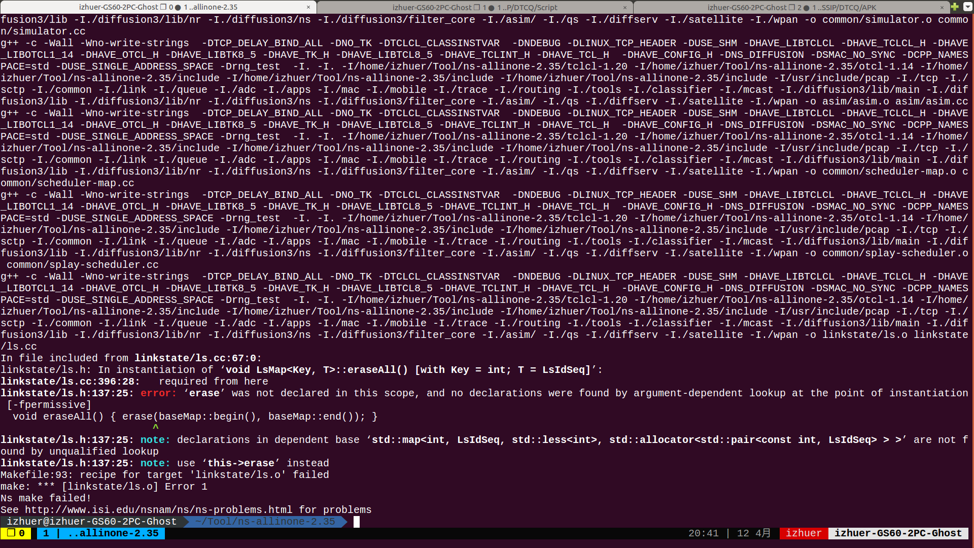
在一筹莫展之际,我在网络上通过 Google 查找了相关文档的信息,最后发现问题是因为 c++ 语法新版和旧版语法不兼容,导致编译出错。考虑到我自身机器就是 Ubuntu,修改 GCC 显然不是明智的决定,于是我对源码进行了修改,经过多次测试以后解决了问题。这也正提醒了我对现实中遇到问题,更应该深入到细节,从根本上发现问题原因并解决。同时也让我更加深信网络资源合理运用的必要性与重要性。
Tcl 语言言网网络环境配置
一、实验目的
利用 tcl 语言建立简单的场景,满足:
- 圆上的 n 个点,n 由用户输入。
- CBR数据流对角节点(如节点 1 和节点 7)之间简单的数据流。
二、实验内容
- 阅读和理解参考代码;
- 根据参考代码完成 circle.tcl 文件,接受用户输入 n ,建立通信场景,满足通信节点为圆上等距分布的 n 个点,且对角节点之间传送简单数据流。
三、实验步骤及测试结果
- 完整代码(circle.tcl)如下:
# editingset val(stop) 100set val(tr) out.tr#设定模拟需要的一些属性set val(chan) Channel/WirelessChannelset val(prop) Propagation/TwoRayGroundset val(netif) Phy/WirelessPhyset val(mac) Mac/802_11#将协议设置为 DSR 后,同时将队列设置为 CMUPriQueueset val(ifq) CMUPriQueueset val(ll) LLset val(ant) Antenna/OmniAntennaset val(ifqlen) 50#将结点个数预设为 0,待用户输入。此项要求用户一定输入,否则不执行模拟。set val(nn) 0set val(rp) DSR#场景大小缺省值为 1000*1000set val(x) 1000set val(y) 1000#圆的半径缺省值为 400set val(r) 300#该过程用于在屏幕上打印在终端输入 ns circle.tcl 后添加参数的格式proc usage {} {global argv0puts "\nusage: $argv0 \[-nn nodes\] \[-r r\] \[-x x\] \[-y y\]\n"puts "note: \[-nn nodes\] is essential, and the others are optional.\n"}#该过程用来根据用户的输入更改一些预设参数的值proc getval {argc argv} {# editingglobal vallappend vallist r x y z#argc 为参数的个数,argv 为整条参数构成的字符串for {set i 0} {$i < $argc} {incr i} {#变量 arg 为 argv 的第 i 部分,以空格为分界set arg [lindex $argv $i]#略过无字符“-”的字符串,一般是用户键入的数字#string range $arg m n 表示取字符串$arg 的第 m 个字符到第 n 个字符if {[string range $arg 0 0] != "-"} continueset name [string range $arg 1 end]#更改预设变量(结点个数,半径,场景大小)set val($name) [lindex $argv [expr $i+1]]}}#调用 getval 过程getval $argc $argv#用户没有输入参数,只键入了 ns circle.tcl,则结点个数认为 0if { $val(nn) == 0 } {#打印用法usageexit}#初始化全局变量set ns [new Simulator]#打开 Trace 文件set namfd [open ns1.nam w]$ns namtrace-all-wireless $namfd $val(x) $val(y)set tracefd [open $val(tr) w]$ns trace-all $tracefd#建立一个拓扑对象,以记录移动节点在拓扑内移动的情况set topo [new Topography]#拓扑范围为 1000m*1000m$topo load_flatgrid $val(x) $val(y)#创建物理信道对象set chan [new $val(chan)]#创建 God 对象set god [create-god $val(nn)]#设置移动节点属性$ns node-config -adhocRouting $val(rp) \-llType $val(ll) \-macType $val(mac)\-ifqType $val(ifq) \-ifqLen $val(ifqlen) \-antType $val(ant) \-propType $val(prop) \-phyType $val(netif)\-channel $chan \-topoInstance $topo \-agentTrace ON \-routerTrace ON \-macTrace OFF \-movementTrace ONfor {set i 0} {$i < $val(nn)} {incr i} {set node_($i) [$ns node]}#设定移动节点的初始位置(提示:通过三角函数实现节点数未知情况下的节点位置设置)# editingset angle [expr 3.1415926535897932384626433832795021141979 * 2 / $val(nn)]for {set i 0} {$i < $val(nn)} {incr i} {$node_($i) set X_ [expr cos($angle * $i) * $val(r) + $val(r)]$node_($i) set Y_ [expr sin($angle * $i) * $val(r) + $val(r)]$node_($i) set Z_ 0}#新建一个 UDP Agent 并把它绑定到节点 1 上# editingset udp0 [new Agent/UDP]$ns attach-agent $node_(1) $udp0##新建一个 CBR 流量发生器,设定分组大小为 500Byte,发送间隔为 5ms,然后绑定到 udp0 上# editingset cbr0 [new Application/Traffic/CBR]$cbr0 set packetSize_ 500$cbr0 set interval_ 0.005$cbr0 attach-agent $udp0#在 node_(1)节点沿直径对面的节点上建立一个数据接受器(对面节点号需要计算)# editingset faceid [expr ($val(nn) / 2 + 1) % $val(nn)]set null0 [new Agent/Null]$ns attach-agent $node_($faceid) $null0#将这两个 Agent 连接起来# editing$ns connect $udp0 $null0$ns at 0.5 "$cbr0 start"$ns at 4.5 "$cbr0 stop"#在 Nam 中定义节点初始所在位置for {set i 0 } {$i<$val(nn)} {incr i} {#只有定义了移动模型后,这个函数才能被调用$ns initial_node_pos $node_($i) 30}#定义节点模拟的结束时间# editingfor {set i 0 } {$i<$val(nn)} {incr i} {$ns at $val(stop) "$node_($i) reset";}$ns at $val(stop) "stop"$ns at $val(stop) "puts \"NS EXITING...\"; $ns halt"#stop 函数proc stop {} {global ns tracefd namfd$ns flush-traceclose $tracefdclose $namfdexec nam ns1.nam &}$ns run
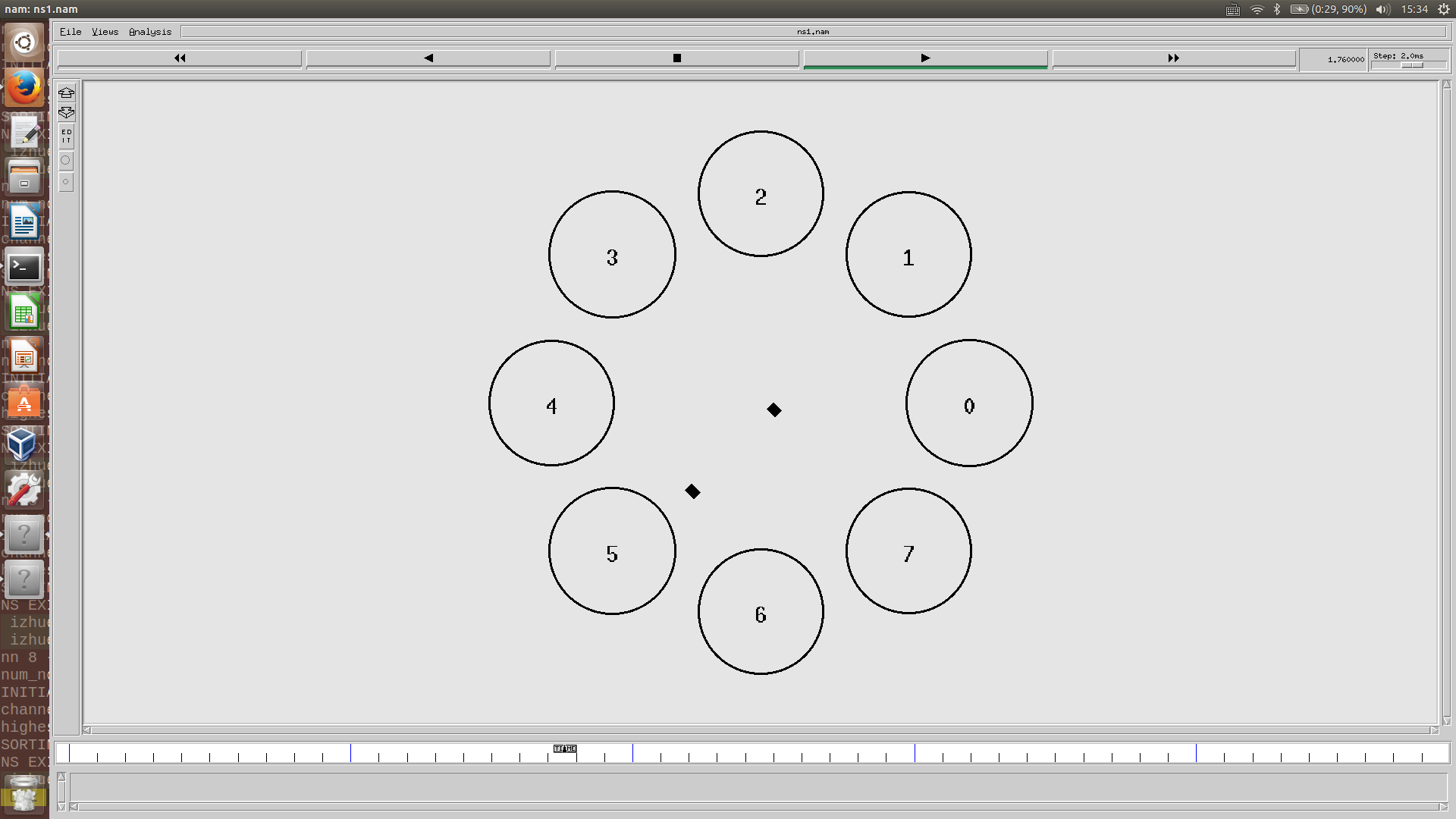
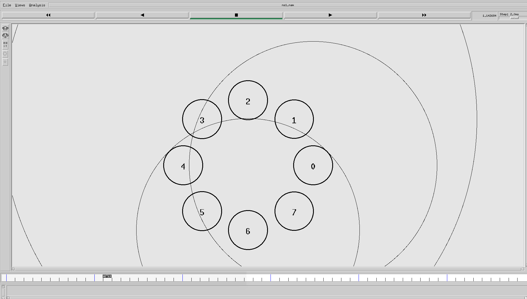
测试结果如下:
ns two_circle.tcl -nn 8 -x 100 -y 100 -r 50 (n 取 8,圆半径为 50,1 和 5 可以直接传递数据)
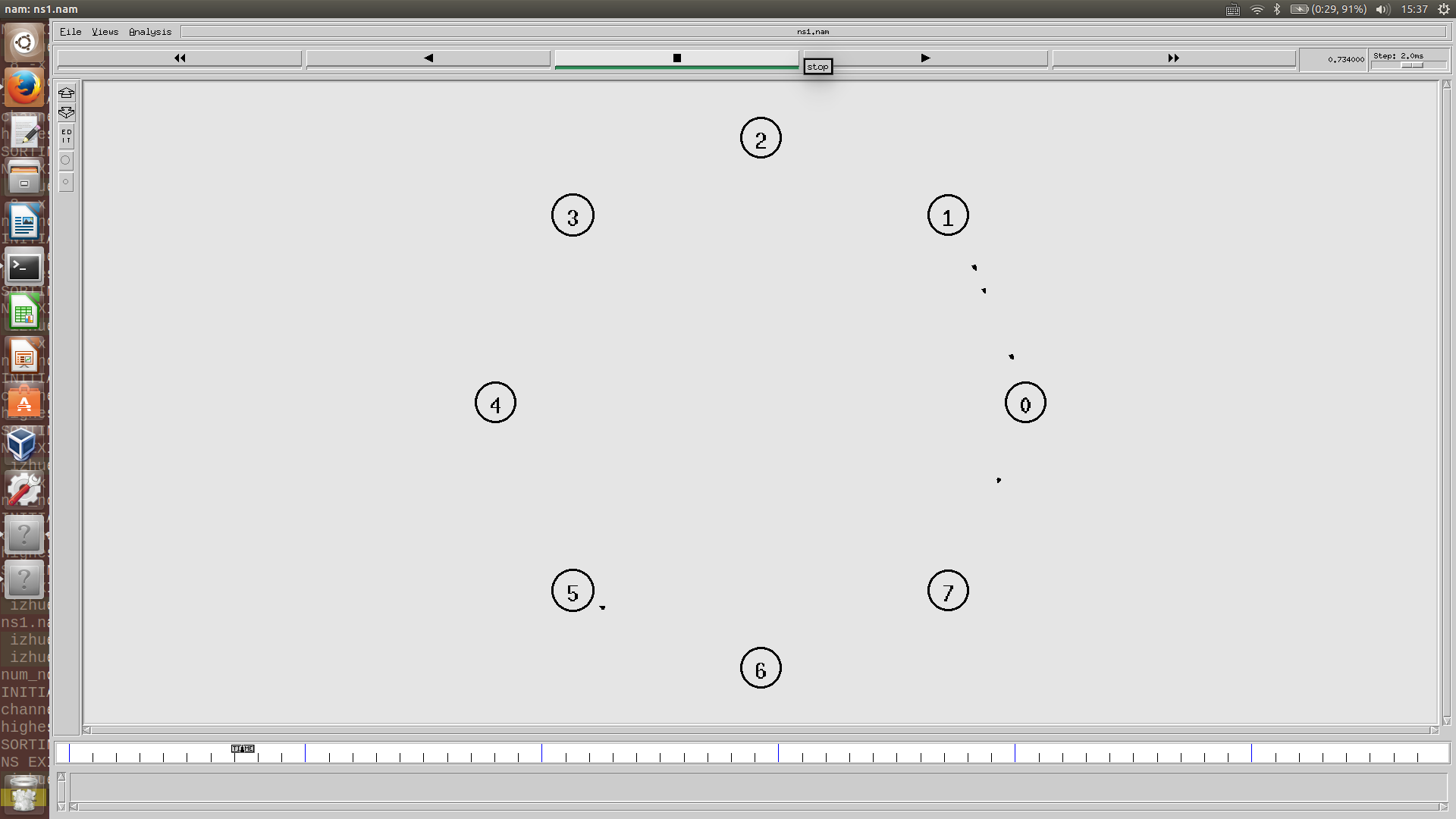
ns two_circle.tcl -nn 8 -x 100 -y 100 -r 200 (n 取 8,圆半径为 200, 1 和 5 需要间接传递数据)
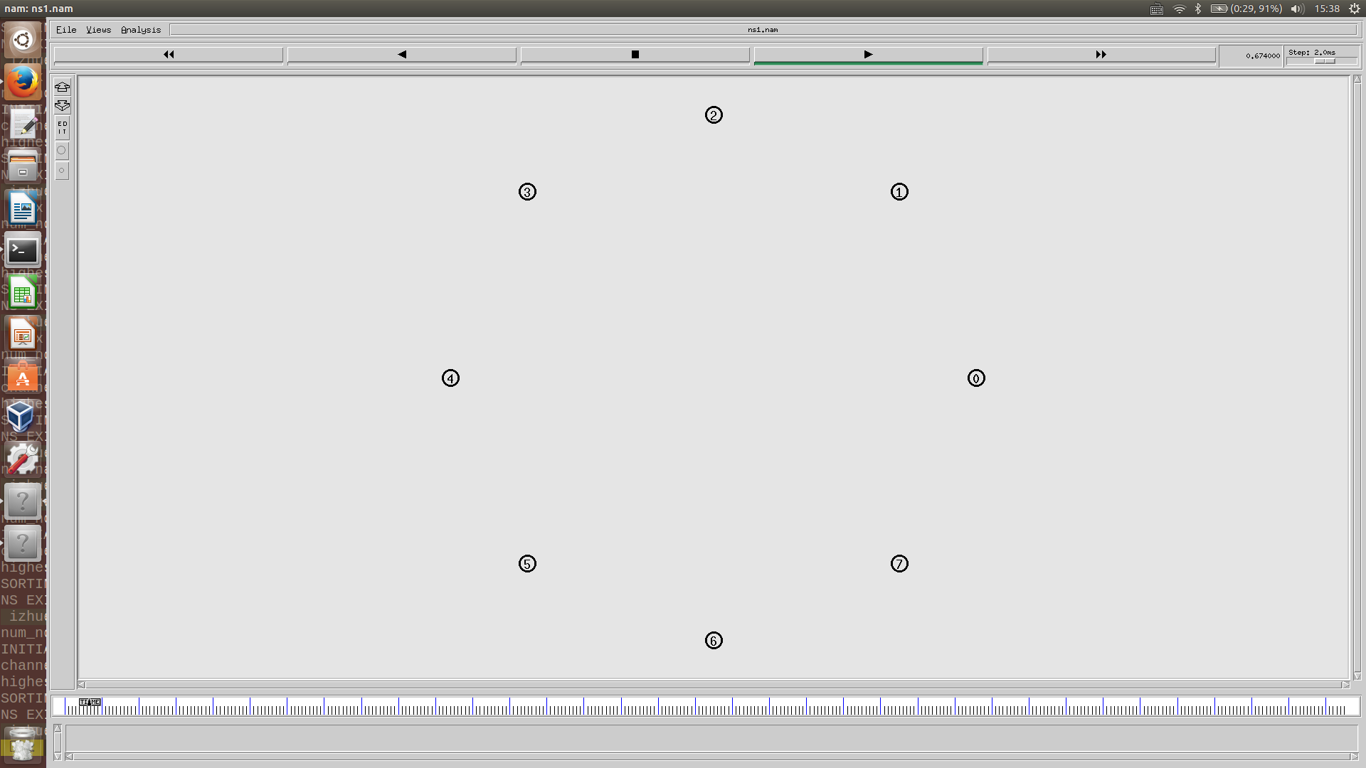
ns two_circle.tcl -nn 8 -x 100 -y 100 -r 500 (n 取 8,圆半径为 500, 1 和 5 无法传递数据)
四、实验心得与体会
在实验过程中,首先我体会到了 Tcl 语言和我熟悉的语言的不同之处。Tcl 语言和 C 语言在语法上有着很大的差异性,有时候在短时间内无法习惯过来,不过后来发现和 Bash 脚本语言很相像,渐渐找到了书写的感觉。另一方面,模拟实验也让我生动地感受到了节点数据传输的原理,在通信数据的传输过程中,节点间都倾向于直接传递数据,所以在半径为五十的情况下节点一和节点五可以直接交互。但是如果节点间的距离过大,数据传输就会经过其他节点,正如半径为两百时的情况。而最后,像半径为五百时,当节点距离达到相邻节点都无法传输数据时,传输就会失败。
使用用CMU工工具配置一一个随机场景
一、实验目的
- 学习使用 CMU 工具生成随机节点场景及 CBR 数据流。
- 学习使用 gawk 工具分析模拟结果。
二、实验内容
setdest 和 cbrgen 是 CMU(卡内基梅隆大学)开发的用于生成无线节点移动场景和随机 cbr 数据流的工具。例如 ./setdest -n 100 -p 5 -M 2 -t 3600 -x 1000 -y 1000 > my_scene.txt 的含义是生成一个 100 个节点以最大速度 2m/s 的速度在大小为 1000m*1000m 的区域内随机运动 1 小时(3600 秒)每到达一个地方停留 5 秒的无线节点移动的场景,场景文件重定向到文件 my_scene.txt 中。
gawk 是用来分析 Trace 文件的工具。而使用 gawk 非常简单只需要将用 gawk 语言写好
的用以分析对应的 Trace 文件的脚本放在 Trace 文件所在的目录下,通过命令“gawk –f xxx.awk xxx.tr”就可以使用 gawk 来分析 Trace 文件。其中,xxx.awk 就是用以分析 Trace 文件的 gawk 脚本。xxx.tr 就是所需要分析的 Trace 文件。本次实验需要完成 random.tcl 文件和 RandomScene.tcl 文件,使用gawk对模拟结果进行分析。
三、实验步骤及测试结果
- run.tcl 文件代码如下:
set seed [exec ./RandomNumber] ;#get a random number as seedputs "seed is $seed"puts "creating 50 random nodes"# editingexec /home/izhuer/Tool/ns-allinone-2.35/ns-2.35/indep-utils/cmu-scen-gen/setdest/setdest -n 50 -p 5 -M 2 -t 3600 -x 900 -y 900 > RandomDest.txt#create 50 random nodes by setdest, output to file RandomDest.txt; The route depends on different computers.puts "creatingnodes done"puts "creating random cbr stream"# editingexec ns /home/izhuer/Tool/ns-allinone-2.35/ns-2.35/indep-utils/cmu-scen-gen/cbrgen.tcl -type cbr -nn 50 -seed $seed -mc 25 -rate 1.0 > RandomCbr.txt#create 50 nodes' random cbr stream by cbrgen.tcl, output to file RandomCbr.txt; The route depends on different computers.puts "creating cbr stream done\n"puts "-------------Simulation-------------"source RandomScene.tcl ; #run simulatior
- 用来获得随机种子的 RandomNumber.cc 文件代码如下:
#include <iostream>#include <cstdlib>#include <ctime>using namespace std;int main(){unsigned int num = (unsigned)time(NULL);cout<<num<<endl;return 0;}
- RandomScene.tcl 的代码如下:
Phy/WirelessPhy set RXThresh_ 2.28289e-11 ;# set valid wirless connection distance is 500mset val(chan) Channel/WirelessChannel ;# channel typeset val(prop) Propagation/TwoRayGround ;# radio-propagation modelset val(netif) Phy/WirelessPhy ;# network interface typeset val(mac) Mac/802_11 ;# MAC typeset val(ifq) CMUPriQueue ;# interface queue typeset val(ll) LL ;# link layer typeset val(ant) Antenna/OmniAntenna ;# antenna modelset val(ifqlen) 50 ;# max packet in ifqset val(nn) 50 ;# number of mobile nodesset val(rp) DSR ;# routing protocolset val(x) 900 ;# X dimensions of the topographyset val(y) 900 ;# X dimensions of the topographyset val(ncbr) 25 ;# number of cbr streams#set up a global instance of Simulatorset ns_ [new Simulator]#open files to record the simulation resultsset tracefd [open RandomScene.tr w]$ns_ trace-all $tracefdset namtracefd [open RandomScene.nam w]$ns_ namtrace-all-wireless $namtracefd $val(x) $val(y)#a function called in proc finish to analyse trace and print result# editingproc analysis {} {puts ""puts "-------------Analysis-------------"puts [exec gawk -f three.awk RandomScene.tr]}#a function called at the end of the simulation to close the recording files and show the animation# editingproc finish {} {global ns_ tracefd namtracefd$ns_ flush-traceclose $tracefdclose $namtracefdanalysisexec nam RandomScene.nam &$ns_ halt}#set up the topography of the sceneset topo [new Topography]$topo load_flatgrid $val(x) $val(y)#set up a global instance of Godset god_ [create-god $val(nn)]#configure all the nodes in the simulation using variables initialized at the beginning$ns_ node-config -addressType def \-adhocRouting $val(rp) \-llType $val(ll) \-macType $val(mac) \-ifqType $val(ifq) \-ifqLen $val(ifqlen) \-antType $val(ant) \-propType $val(prop) \-phyType $val(netif) \-channelType $val(chan) \-topoInstance $topo \-agentTrace ON \-routerTrace ON \-macTrace OFF \-movementTrace OFF#set up nodes and disable their functions of random motionfor {set i 0} {$i<$val(nn)} {incr i} {set node_($i) [$ns_ node]$node_($i) random-motion 0}source RandomDest.txtsource RandomCbr.txt#stop all the cbr streams from generating packetsfor {set i 0} {$i < $val(ncbr)} {incr i} {$ns_ at 50.0 "$cbr_($i) stop"}#reset all the nodesfor {set i 0} {$i<$val(nn)} {incr i} {$ns_ at 50.0 "$node_($i) reset"}#call function "finish" to close files and show the animation$ns_ at 60.0 "finish"#run the simulation$ns_ run
- 用于分析 trace 文件的 three.awk 脚本代码如下:
BEGIN {#设置初始变量num_D = 0; #丢包数num_s = 0; #发送包数num_r = 0; #收到包数rate_drop=0; #丢包率sum_delay=0; #总延迟时间average_delay=0; #平均延迟时间}{#读取 trace 文件记录event = $1; #第一列为包的操作(s 为发送包,r 为接受包)time = $2; #第二列为操作时间node=$3; #第三列为节点号trace_type = $4; #第四列为操作层flag = $5; #第五列为标志位uid = $6; #第六列为pkt_type = $7; #第七列为包类型pkt_size = $8; #第八列为包的大小#操作if (event== "s" && trace_type== "AGT" && pkt_type== "cbr"){ send_time[uid]=time; #创建数组记录发包时间num_s++;#记录发送包总数}if (event== "r" && trace_type== "AGT" && pkt_type== "cbr"){ delay[uid]=time-send_time[uid]; #创建数组记录延迟时间num_r++; #记录收到包总数}if (event== "D" && pkt_type== "cbr")delay[uid]=-1; #-1 表示包丢失, 该包不会记入延迟时间}END {#计算丢包数和丢包率num_D = num_s-num_r; #丢包总数rate_drop=num_D/num_s*100.0; #计算丢包率#计算延迟for(i=0;i<num_s;i++){if(delay[i]>=0)sum_delay+=delay[i];}#总延迟时间average_delay=sum_delay/num_r;#平均延迟时间#打印结果printf("number of packets droped:%d \n",num_D);printf("number of packets sent:%d \n",num_s);printf("drop rate:%.3f%% \n",rate_drop );printf("average delay time:%.9f \n",average_delay );}
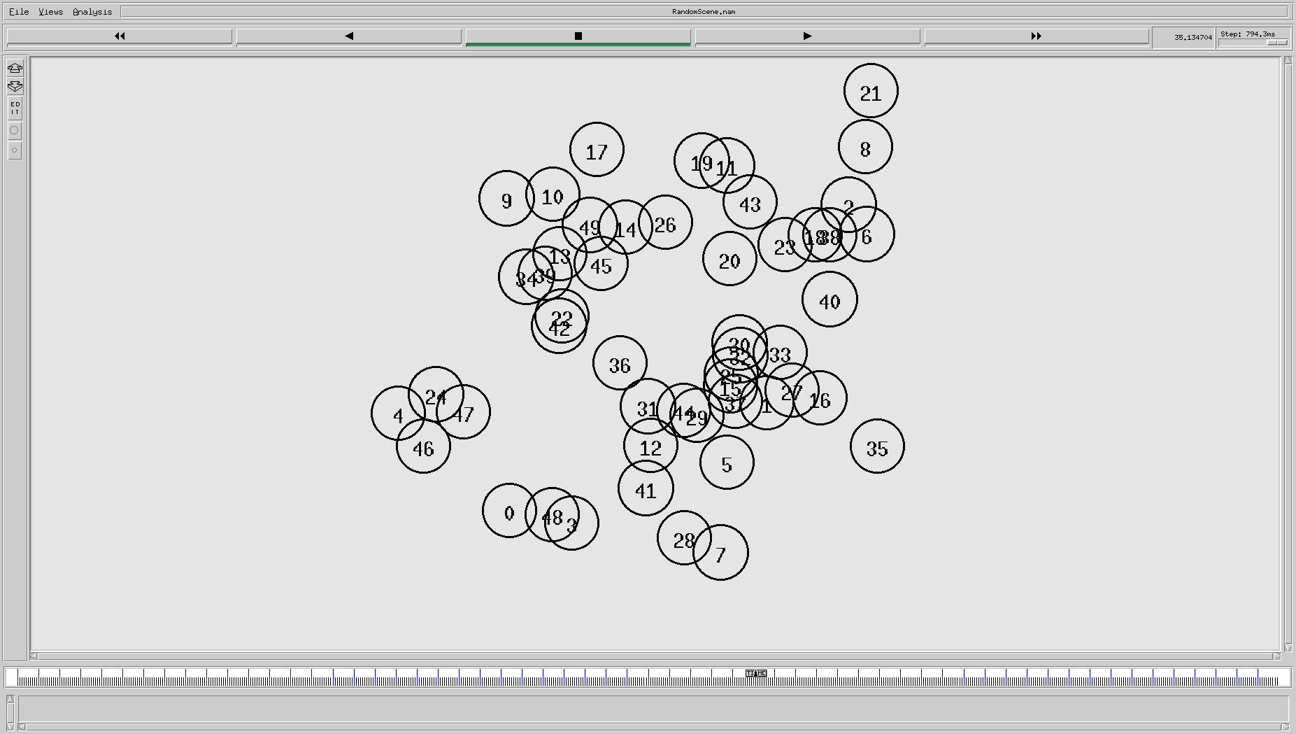
nam模拟结果如下图所示:
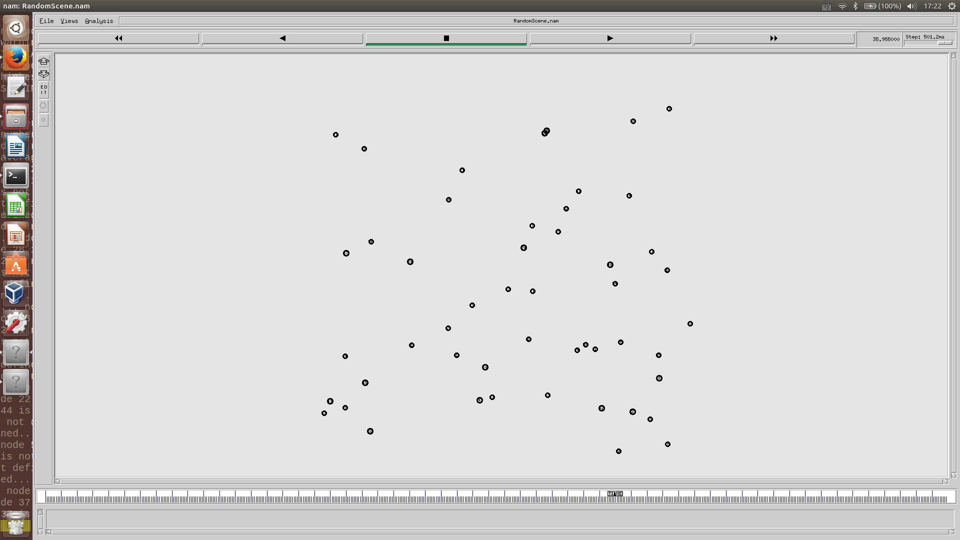
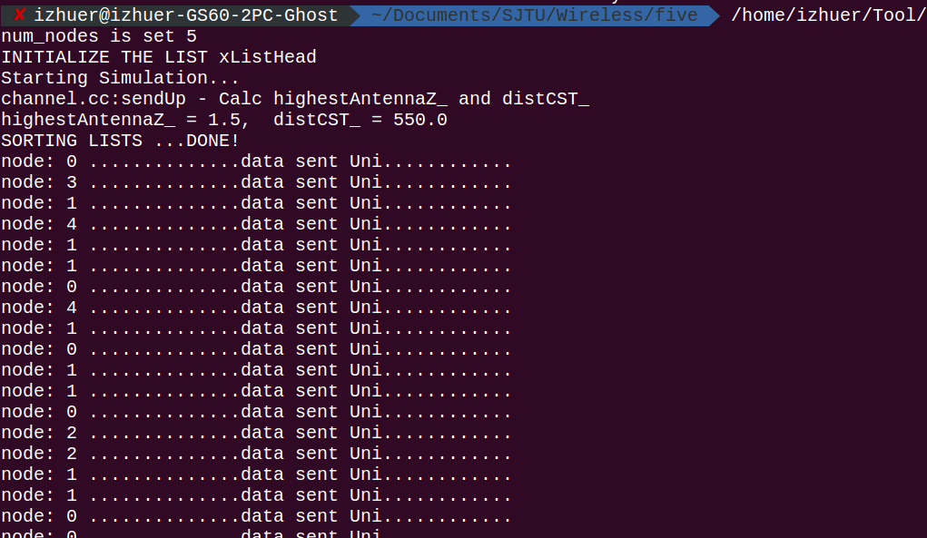
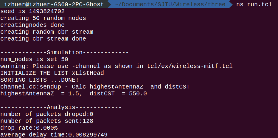
gawk 分析结果如下所示:
seed is 1492075896creating 50 random nodescreatingnodes donecreating random cbr streamcreating cbr stream done-------------Simulation-------------num_nodes is set 50warning: Please use -channel as shown in tcl/ex/wireless-mitf.tclINITIALIZE THE LIST xListHeadchannel.cc:sendUp - Calc highestAntennaZ_ and distCST_highestAntennaZ_ = 1.5, distCST_ = 550.0SORTING LISTS ...DONE!-------------Analysis-------------number of packets droped:0number of packets sent:184drop rate:0.000%average delay time:0.008996461
四、实验心得与体会
在这次实验的过程中,我发现丢包率与分组的发送率还是有着一定的关系的。在我们的实验数据中,我设置分组发送率为 1.0 时,丢包率为 0,而当我设置分组发送率为 100.0 时,我们得到了如下的实验结果:
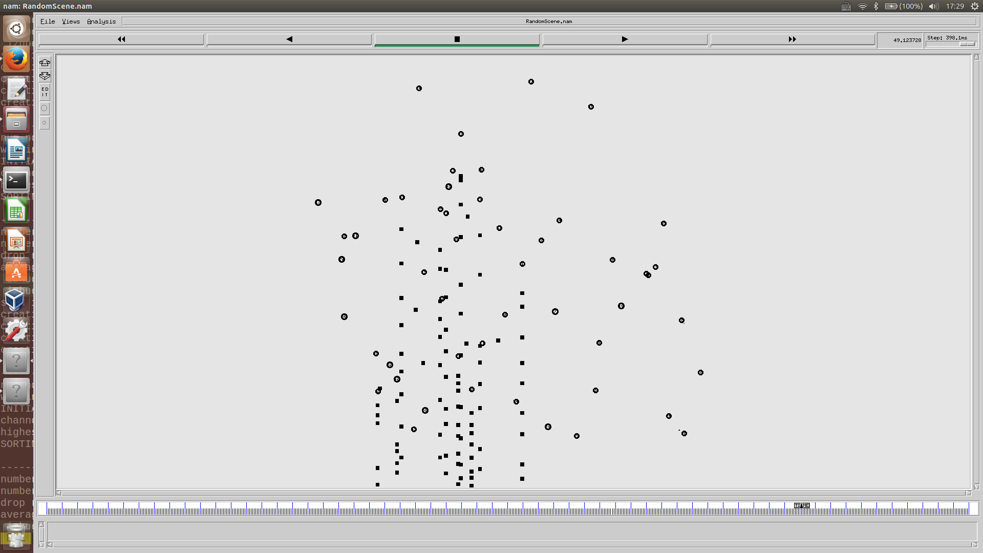
我们可以看到,这里有着大量的数据包丢失,然后我们在从 gawk 的数据中去分析:
seed is 1492075746creating 50 random nodescreatingnodes donecreating random cbr streamcreating cbr stream done-------------Simulation-------------num_nodes is set 50warning: Please use -channel as shown in tcl/ex/wireless-mitf.tclINITIALIZE THE LIST xListHeadchannel.cc:sendUp - Calc highestAntennaZ_ and distCST_highestAntennaZ_ = 1.5, distCST_ = 550.0SORTING LISTS ...DONE!-------------Analysis-------------number of packets droped:17766number of packets sent:23496drop rate:75.613%average delay time:0.719766833
我们会发现,丢包率已经达到了 76% 之高,这也从实验上证明了我们的猜测。也就是说,在显示生活中,我们移动通信还需要着重关注负载平衡,不能一味提高发送率。
在NS2中移植实现MFLood协议
一、实验目的
- 将 MFlood 路由协议添加到 NS-2 中(MFlood 协议是一个很简单的路由协议,每个节点在收到目的不是自己的包后就将其广播出去,但不会重复广播同一个包);
- 使用随机场景脚本进行测试
二、实验原理
一般而言, 在 NS-2 中移植协议主要有以下几步:
- 添加新的代码文件。这些文件就是对协议进行描述的一些都文件和源文件,录入 protocol.h 和 protocol.cc 等。我们可以在 ns-allinone-~ns/~ns 目录下新建一个 protocol 的文件夹来存放这些文件,有时我们也会将他们放置在已有的文件夹下。
- 修改 NS-2 原有的一些文件。由于新添加的协议会用到一些 NS-2 已有的类,结构或者变量,可能会对 NS-2 中一些原有的信息进行更改或者扩。例如,新的协议可能会有它自己的协议头和消息类型,那么需要对 NS-2 定义协议头和消息类型的那些文件进行修改,添加必要的内容。不同的协议需要修改的文件不同,这是由新协议需要描述的内容决定的。通常需要修改的文件有:定义消息类型和普通头部的文件 packet.h 、定义分组头部的文件 ns-packet.tcl 、定义默认参数的文件 ns-default.tcl 等。
- 修改 NS-2 的 Makefile 文件。我们编写完描述协议的代码以后,需要将它们整合到 NS-2 中,称为 NS-2 中的一部分。而修改 Makefile 文件就是整合的过程。
三、实验内容
- 添加新的代码文件
- 修改 NS-2 原有的一些文件
- 修改 NS-2 的 Makefile 文件
- 验证移植结果
四、实验步骤及测试结果
在ns-allinone-2.35/ns-2.35目录下新建文件夹mflood,将文件mflood.h, mflood.cc, mflood_packet.h, mflood-seqtable.h, mflood-seqtable.cc放置于 mflood 文件夹中;

修改文件/common/packet.h
......static const packet_t PT_MFLOOD = 73;static packet_t PT_NTYPE = 74; // This MUST be the LAST one.....name_[PT_MFLOOD] = "MFlood";name_[PT_NTYPE]= "undefined";
- 修改文件/tcl/lib/ns-packet.tcl
# Mobility, Ad-Hoc Networks, Sensor Nets:AODV # routing protocol for ad-hoc networksMFloodDiffusion # diffusion/diffusion.ccIMEP # Internet MANET Encapsulation Protocol, for ad-hoc networksMIP # Mobile IP, mobile/mip-reg.ccSmac # Sensor-MACTORA # routing protocol for ad-hoc networksMDART # routing protocol for ad-hoc networks# AOMDV patchAOMDV
- 修改文件/tcl/lib/ns-lib.tcl
......AODV {set ragent [$self create-aodv-agent $node]}MFlood {set ragent [$self create-mflood-agent $node]}AOMDV {set ragent [$self create-aomdv-agent $node]}......Simulator instproc create-aodv-agent { node } {# Create AODV routing agentset ragent [new Agent/AODV [$node node-addr]]$self at 0.0 "$ragent start" ;# start BEACON/HELLO Messages$node set ragent_ $ragentreturn $ragent}Simulator instproc create-mflood-agent { node } {set ragent [new Agent/MFlood [$node id]]$node set ragent_ $ragentreturn $ragent}
- 修改Makefile
......aodv/aodv_logs.o aodv/aodv.o \aodv/aodv_rtable.o aodv/aodv_rqueue.o \mflood/mflood.o mflood/mflood-seqtable.o \aomdv/aomdv_logs.o aomdv/aomdv.o \aomdv/aomdv_rtable.o aomdv/aomdv_rqueue.o \......
- 重新编译 NS-2并修改实验一中的场景
# editingset val(stop) 100set val(tr) out.tr#设定模拟需要的一些属性set val(chan) Channel/WirelessChannelset val(prop) Propagation/TwoRayGroundset val(netif) Phy/WirelessPhyset val(mac) Mac/802_11#将协议设置为 DSR 后,同时将队列设置为 CMUPriQueueset val(ifq) CMUPriQueueset val(ll) LLset val(ant) Antenna/OmniAntennaset val(ifqlen) 50#将结点个数预设为 0,待用户输入。此项要求用户一定输入,否则不执行模拟。set val(nn) 0set val(rp) MFlood......
输出信息:
ns two_circle.tcl -nn 8 -r 50 -x 100 -y 100num_nodes is set 8INITIALIZE THE LIST xListHead5channel.cc:sendUp - Calc highestAntennaZ_ and distCST_highestAntennaZ_ = 1.5, distCST_ = 550.0SORTING LISTS ...DONE!NS EXITING...
弹出运行截图:
为了更加清晰地展示输出信息,我查看了节点 3 的 trace:
grep "^[fr]*_3" out.tr......r 5.598748669 _3_ RTR --- 430 cbr 520 [0 ffffffff 6 800] ------- [1:0 5:0 29 0] [430] 2 0f 5.599054615 _3_ RTR --- 431 cbr 520 [0 ffffffff 1 800] ------- [1:0 5:0 29 0] [431] 1 0r 5.608621336 _3_ RTR --- 426 cbr 520 [0 ffffffff 7 800] ------- [1:0 5:0 29 0] [426] 2 0r 5.613315438 _3_ RTR --- 430 cbr 520 [0 ffffffff 0 800] ------- [1:0 5:0 29 0] [430] 2 0r 5.618009591 _3_ RTR --- 429 cbr 520 [0 ffffffff 4 800] ------- [1:0 5:0 29 0] [429] 2 0r 5.622763827 _3_ RTR --- 430 cbr 520 [0 ffffffff 2 800] ------- [1:0 5:0 29 0] [430] 2 0r 5.632212298 _3_ RTR --- 432 cbr 520 [0 ffffffff 1 800] ------- [1:0 5:0 30 0] [432] 1 0r 5.636946498 _3_ RTR --- 430 cbr 520 [0 ffffffff 4 800] ------- [1:0 5:0 29 0] [430] 2 0r 5.641661012 _3_ RTR --- 429 cbr 520 [0 ffffffff 7 800] ------- [1:0 5:0 29 0] [429] 2 0f 5.642938569 _3_ RTR --- 432 cbr 520 [0 ffffffff 1 800] ------- [1:0 5:0 29 0] [432] 1 0r 5.646375114 _3_ RTR --- 431 cbr 520 [0 ffffffff 0 800] ------- [1:0 5:0 29 0] [431] 2 0r 5.651109169 _3_ RTR --- 431 cbr 520 [0 ffffffff 2 800] ------- [1:0 5:0 29 0] [431] 2 0r 5.655803683 _3_ RTR --- 431 cbr 520 [0 ffffffff 6 800] ------- [1:0 5:0 29 0] [431] 2 0r 5.660557919 _3_ RTR --- 433 cbr 520 [0 ffffffff 1 800] ------- [1:0 5:0 30 0] [433] 1 0r 5.670330585 _3_ RTR --- 431 cbr 520 [0 ffffffff 7 800] ------- [1:0 5:0 29 0] [431] 2 0r 5.675024688 _3_ RTR --- 432 cbr 520 [0 ffffffff 0 800] ------- [1:0 5:0 29 0] [432] 2 0f 5.675377768 _3_ RTR --- 433 cbr 520 [0 ffffffff 1 800] ------- [1:0 5:0 29 0] [433] 1 0r 5.679718841 _3_ RTR --- 432 cbr 520 [0 ffffffff 7 800] ------- [1:0 5:0 29 0] [432] 2 0r 5.684492943 _3_ RTR --- 431 cbr 520 [0 ffffffff 4 800] ------- [1:0 5:0 29 0] [431] 2 0r 5.689307457 _3_ RTR --- 433 cbr 520 [0 ffffffff 0 800] ------- [1:0 5:0 29 0] [433] 2 0r 5.694021512 _3_ RTR --- 432 cbr 520 [0 ffffffff 2 800] ------- [1:0 5:0 29 0] [432] 2 0r 5.698755748 _3_ RTR --- 432 cbr 520 [0 ffffffff 4 800] ------- [1:0 5:0 29 0] [432] 2 0r 5.703450164 _3_ RTR --- 437 cbr 520 [0 ffffffff 1 800] ------- [1:0 5:0 30 0] [437] 1 0r 5.713262830 _3_ RTR --- 433 cbr 520 [0 ffffffff 7 800] ------- [1:0 5:0 29 0] [433] 2 0r 5.717976932 _3_ RTR --- 433 cbr 520 [0 ffffffff 4 800] ------- [1:0 5:0 29 0] [433] 2 0f 5.718399492 _3_ RTR --- 437 cbr 520 [0 ffffffff 1 800] ------- [1:0 5:0 29 0] [437] 1 0r 5.722771446 _3_ RTR --- 437 cbr 520 [0 ffffffff 0 800] ------- [1:0 5:0 29 0] [437] 2 0r 5.727465502 _3_ RTR --- 443 cbr 520 [0 ffffffff 1 800] ------- [1:0 5:0 30 0] [443] 1 0f 5.729130036 _3_ RTR --- 443 cbr 520 [0 ffffffff 1 800] ------- [1:0 5:0 29 0] [443] 1 0r 5.732179882 _3_ RTR --- 437 cbr 520 [0 ffffffff 6 800] ------- [1:0 5:0 29 0] [437] 2 0r 5.741588548 _3_ RTR --- 437 cbr 520 [0 ffffffff 7 800] ------- [1:0 5:0 29 0] [437] 2 0r 5.746282651 _3_ RTR --- 437 cbr 520 [0 ffffffff 4 800] ------- [1:0 5:0 29 0] [437] 2 0r 5.750997067 _3_ RTR --- 443 cbr 520 [0 ffffffff 6 800] ------- [1:0 5:0 29 0] [443] 2 0r 5.755711220 _3_ RTR --- 433 cbr 520 [0 ffffffff 2 800] ------- [1:0 5:0 29 0] [433] 2 0r 5.760505455 _3_ RTR --- 444 cbr 520 [0 ffffffff 1 800] ------- [1:0 5:0 30 0] [444] 1 0f 5.763578769 _3_ RTR --- 444 cbr 520 [0 ffffffff 1 800] ------- [1:0 5:0 29 0] [444] 1 0r 5.765319655 _3_ RTR --- 443 cbr 520 [0 ffffffff 0 800] ------- [1:0 5:0 29 0] [443] 2 0r 5.770033891 _3_ RTR --- 444 cbr 520 [0 ffffffff 6 800] ------- [1:0 5:0 29 0] [444] 2 0r 5.774788044 _3_ RTR --- 443 cbr 520 [0 ffffffff 7 800] ------- [1:0 5:0 29 0] [443] 2 0r 5.794816998 _3_ RTR --- 444 cbr 520 [0 ffffffff 4 800] ------- [1:0 5:0 29 0] [444] 2 0r 5.804305614 _3_ RTR --- 444 cbr 520 [0 ffffffff 0 800] ------- [1:0 5:0 29 0] [444] 2 0r 5.809059669 _3_ RTR --- 444 cbr 520 [0 ffffffff 2 800] ------- [1:0 5:0 29 0] [444] 2 0
我们可以看到,无论是从模拟开始到结束,当模拟场景中的节点收到每个节点在收到目的不是自己的包后就将其广播出去,但同时,它们不会重复广播同一个包。说明 MFlood 协议的移植成功。
五、实验心得与体会
MFlood 洪泛协议是一个简单的无线路由协议,其中基本的思想是:节点根据一定的规则转发自己收到的数据包。协议很简单,协议的移植也不是一个复杂的过程,但是却让我体会到了每一种协议有着各自的长处:洪泛协议虽然简单,看似对各种网络都很有用,但是试考虑对于对于洪泛协议,如果我伪造了一个目的地不存在的报文,那么是不是这个报文会在网络中不停的传递,造成整个网络负载的增大。这只是我的一个猜测,但正是因为这样思维的过程让我对整个洪泛协议有了进一步深入的了解。感谢老师为我们提供这样一个实验机会,也正是因为亲身实践了,我才对这个协议的整个流程有了一些概念性的了解。
在 NS2 协议栈中添加 mac 协议
一、实验目的
- 学习在 ns2 上如何添加一个新的协议(此处定义为 lmac,实现 smac 协议的全部功能)
- 通过在 ns2 仿真我们添加的 lmac 协议,深入理解无线传感网络 smac 协议
二、实验原理
smac 协议简介:
什么是 MAC?即 medium access control,对信道访问的控制协议。 MAC 可以大体分为两大类,scheduled‐based and contention‐based,基于调度的和基于竞争的。scheduled‐based protocol由中心节点分配信道访问,每个节点只能在分得的时刻或者空间访问信道,如 TDMA,CDMA 等就是这样一种协议。contention‐based protocols 是各个节点竞争信道的访问权,竞争胜出者方可访问信道,CSMA 是其典型代表。这两种协议方式各有优缺点,花开两朵,各表一枝。基于调度的以后再论,先说这基于竞争的。主要特点有:
- 拓扑变化具有适应性,具有可扩展性。
- 用于 multi‐hop 网络。
- 不需要严格同步。
- 会发生碰撞。
- 存在较为严重的隐藏终端问题(idden terminal problems)。
SMAC 就是一种基于竞争的协议,但是又因为它适应于 WSN,与传统的无线网络协议有所不同。Energy conservation and self‐configuation are primary goals,while per‐node fairness and latency are less important。要节约能耗,必须先了解能量浪费的来源:
- ollision,碰撞, 当节点 B 在和节点 A 通信时,不可以和节点 C 同时通信,否则和节点 A 的通信也会遭到破坏,这就是碰撞,碰撞要求重传,重传会引发能耗消耗。
- overheading,串音。当节点 A收到发往其他节点发往节点 B 的数据包时,做了无谓的接受工作。
- control packet overhead,控制包的消耗,由于需要大量 RTS,CTS,ACK 等控制包来解决隐藏终端和保证服务质量,所以这些控制包的能量消耗也是很重要的一部分。
- Idle listening,信道监听。
SMAC 采用的机制有周期性的监听和休眠。摒弃传统无线网络节点要么在传输数据要么在监听的特点,采用周期性的休眠机制,使得节点可以减少无谓的监听,在监听时间段内若有数据需要传输则进行数据传输,否则监听时间到后进入休眠这大大节约了能耗,但是也造成了延迟 latency,并且需要同步。
休眠机制的选择。当一个节点广播一个休眠机制时寄希望全网都会采用这个机制,然而由于不同节点可能同时发出机制,所以网内存在几种不同的休眠机制,可采用时间戳和优先级的机制尽可能使得网络同步于一种机制,当然在边界节点(border nodes)可以采用多种机制,可是这样会加快边界节点的能量消耗,不过边界节点的存在对网络拓扑变化有积极的影响,这是因为他们能比其他节点相对更快的检测到新节点的加入。
collision and overheading avoidance,碰撞和串音避免。首先,节点是如何知道网络空闲与否,这里有两种机制,一种是收到其他节点通信的信息,从中可以判断他们通信的时间,故可以设置 NAV,每过一个时间,NAV 减 1,直到为 0,就可判断信道可能空闲。另一种是物理层检测信道信号的强弱来判定,有研究发现检测噪声也可以判断信道的情况。SMAC 采用了碰撞窗口 contention window 来解决碰撞,采用 RTS/CTS 机制来缓解隐藏终端问题和解决串音。有这样原则:相互通信节点 AB 的一跳邻居都不可以在 AB 通信时进行通信。
message passing,数据传输。当需要传输的数据较长时,如果一旦丢失,则需要重传浪费大量能耗。若将其分成小段传输,则需要加入大量控制包。SMAC 采用把数据分成小段并采用一个 RTS /CTS 的方式集中传输数据,当数据丢失时,不同于 802.11 放弃信道重新竞争以保证用户公平性的方法,而是继续占有信道进行重传。这虽然破坏了用户的公平性,但是维护了整体的公平性。
三、实验内容
- 添加新的协议;
- 验证协议是否正确添加成功。
四、实验步骤及测试结果
- 在 ~/Tools/ns-allinone-2.35/ns-2.35/mac 目录下 copy 原来的 smac.cc 和 smac.h
cp smac.cc lmac.cccp smac.h lmac.h
- 打开 lmac.cc 和 lmac.h,把所有的 SMAC 替换成 LMAC,把所有的 smac 替换成 lmac, 把所有的 Smac 替换成 Lmac
用 vim 打开两个文件,在 vim 中执行命令:%s/smac/lmac/g:%s/Smac/Lmac/g
- 在 ~/Tools/ns-allinone-2.35/ns-2.35/common 目录下修改 packet.h
......#define HDR_SMAC(p) ((hdr_smac *)hdr_mac::access(p))#define HDR_LMAC(p) ((hdr_lmac *)hdr_mac::access(p))....// SMAC packetPT_SMAC,// LMAC packetPT_LMAC,...
- 在 ~/Tools/ns-allinone-2.35/ns-2.35/tcl/lib 目录下修改 ns-default.tcl 文件
.....# Turning on/off sleep‐wakeup cycles for SMACMac/SMAC set syncFlag_ 1# Nodes synchronize their schedules in SMACMac/SMAC set selfConfigFlag_ 1# Default duty cycle in SMACMac/SMAC set dutyCycle_ 10#add LMAC here# Turning on/off sleep‐wakeup cycles for LMACMac/LMAC set syncFlag_ 1# Nodes synchronize their schedules in LMACMac/LMAC set selfConfigFlag_ 1# Default duty cycle in LMACMac/LMAC set dutyCycle_ 10.....# Turning on/off sleep‐wakeup cycles for SMACMac/SMAC set syncFlag_ 0# Turning on/off sleep‐wakeup cycles for LMACMac/LMAC set syncFlag_ 0
- 在 ~/Tools/ns-allinone-2.35/ns-2.35/tcl/lib 目录下修改 ns-packet.tcl 文件
.....Lmac # A new Sensor‐MAC....
- 在 ~/Tools/ns-allinone-2.35/ns-2.35/trace 目录下修改 cmu-trace.h
......void format_smac(Packet *p, int offset);void format_lmac(Packet *p, int offset);......
- 修改 cmu-trace.cc 文件
#include<smac.h>#include<lamc.h> // 新加语句......struct hdr_cmn *ch = HDR_CMN(p);struct hdr_ip *ih = HDR_IP(p);struct hdr_mac802_11 *mh;struct hdr_smac *sh;struct hdr_lmac *ph; // 新添加一个指向 lamc 包的指针......char mactype[SMALL_LEN];strcpy(mactype, Simulator::instance().macType());if (strcmp (mactype, "Mac/SMAC") == 0)sh = HDR_SMAC(p);else if (strcmp (mactype,"Mac/LMAC") == 0) // 判断是不是 LMC 包ph = HDR_LMAC(p);elsemh = HDR_MAC802_11(p);......if (strcmp (mactype, "Mac/SMAC") == 0) {format_smac(p, offset);}else if (strcmp (mactype, "Mac/LMAC") == 0) { //新添语句format_lmac(p, offset);}else {format_mac(p, offset);}return;......// mac layer extensionoffset = strlen(pt_‐>buffer());if (strcmp(mactype, "Mac/SMAC") == 0) {format_smac(p, offset);}else if (strcmp(mactype, "Mac/LMAC") == 0) { //新添语句format_lmac(p, offset);}else {format_mac(p, offset);}......(ch‐>ptype() == PT_SMAC) ? ((sh‐>type == RTS_PKT) ? "RTS" : //新添语句(sh‐>type == RTS_PKT) ? "RTS" :(sh‐>type == CTS_PKT) ? "CTS" :(sh‐>type == ACK_PKT) ? "ACK" :(sh‐>type == SYNC_PKT) ? "SYNC" : "UNKN") :p acket_info.name(ch‐>ptype())), ch‐>size());......void CMUTrace::format_lmac(Packet *p, int offset) //加入函数{struct hdr_lmac *ph = HDR_LMAC(p);sprintf(pt_‐>buffer() + offset, " [%.2f %d %d] ",ph‐>duration,ph‐>dstAddr,ph‐>srcAddr);}.....switch(ch‐>ptype()) {case PT_MAC:case PT_SMAC:case PT_LMAC: //这是新添加的 LMAC 协议break;case PT_ARP:format_arp(p, offset);break;
查找 smac.h 和 lmac.h,有相同类、函数、变量声明时,把 lmac.h 中 与 smac.h 重名的声明改成其它名字,当然在 lmac.cc 中要做相应的修改
在 ~/Tools/ns-allinone-2.35/ns-2.35/ 目录下修改 Makefile 文件
......mac/mac‐802_3.o mac/mac‐tdma.o mac/smac.o mac/lmac.o\......
- 重新 make 编译 ns
cd ~/Tools/ns-allinone-2.35/sudo ./install
- 运行结果
用新编译出来的 ns 对 lmac.tcl 进行运行,运行 nam 如下:
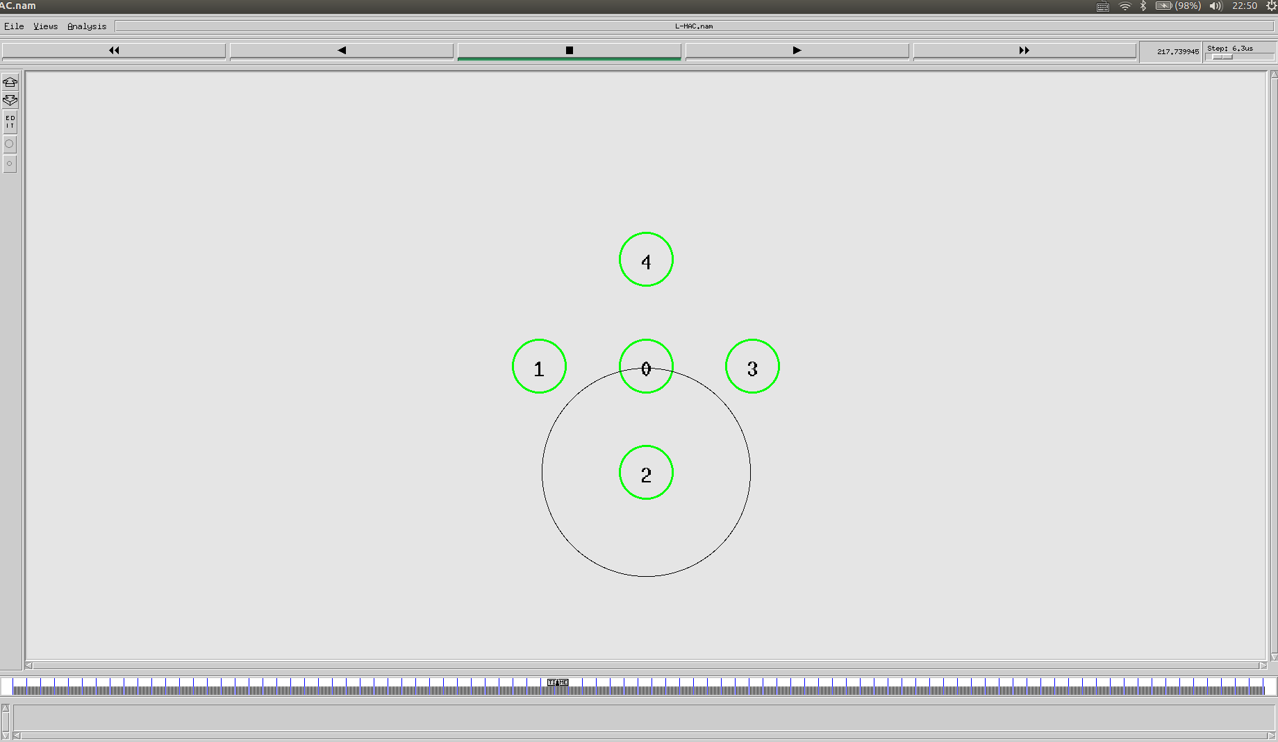
运行的命令行结果如下:
另外,运行 smac.tcl,将生成的两个 trace 文件进行 diff 比对,发现文件一致,说明 lmac 协议添加成功:

五、实验心得与体会
这次实验我遇到了不小的问题,主要在于 Lmac 和 Smac 这两个代码容易混淆,经常编译通过以后不能正常运行 lamc.tcl 文件,反反复复很多次以后终于通过了编译。另外一个遇到的问题是按照教材里说的:
make cleanmake dependmake
每次都无法正常通过编译,最后我是通过直接 install 整个文件去解决的这个问题的。好在有了前面移植 Mflood 协议的经验,我才顺利的完成了这个实验。
另外,通过 Smac 的协议讲解,我也意识到了这是一个非常节省网络通讯压力的协议。在 Smac 下,每个节点不必一直处于监听状态,就从监听这个方面减轻了网路的负载。但是反过来,这也导致了网络的延迟,有利必有弊,我从 MFlood 到 Smac 中深刻认识到网络协议的发展就是不断地在性能和效率中权衡取最优值,最终目标就是达到一个适合整个网络的平衡态。
无线自组织网络 AODV 协议的仿真
一、实验目的
在 NS-2 仿真 AODV 协议,并在 trace 文件中了解 AODV 协议的原理。
二、实验原理
- AODV 简介
AODV 是由 Nokia 研究中心的 CharlesE.Perkins 和加利福尼亚大学 SantaBarbara的 ElizabethM.Belding-Roryer 以及 Cincinnati 大学 SamirR.Das 等共同开发,已经被IETFMANET 工作组于 2003 年 7 月正式公布为自组网路由协议的 RFc 标准。AODV实质上就是 DSR 和 DSDV 的综合,它借用了 DSR 中路由发现和路由维护的基础程序,及 DSDV 的逐跳 (Hop-by-Hop)路由、目的节点序列号和路由维护阶段的周期更新机制,以 DSDV 为基础,结 合 DSR 中的按需路由思想并加以改进。
AODV 在每个中间节点隐式保存了路由请求和应答的结果,并利用扩展环搜索的办法 来限制搜索发现过的目的节点的范围。AODV 支持组播功能,支持 QoS,而且 AODV 中可 以使用 IP地址,实现同 Internet 连接,但是不支持单向信道。和 DSDV 保存完整的路由表 不同的是,AODV 通过建立基于按需路由来减少路由广播的次数,这是 AODV 对 DSDV的 重要改进。和 DSR 相比,AODV 的好处在于源路由并不需要包括在每一个数据分组中,这样会使路由协议的开销有所降低。AODV 是一个纯粹的按需路由系统,那些不在路径内的 节点不保存路由信息,也不参与路由表的交换。AODV 协议可以实现在移动终端间动态的、 自发的路由,使移动终端很快获得通向所需目的的路由,同时又不用维护当前没有使用的路 由信息,并且还能很快对断链的拓扑变化做出反应。AODV 的操作是无环路的,在避免了 通常 Bellman-ford 算法的无穷计数问题的同时,还提供了很快的收敛速度。AODV 的路由表 中每个项都使用了目的序列号(DestinationSequenceNumber)。目的序列号是目的节点创建, 并在发给发起节点的路由信息中使用的。使用目的序列号可以避免环路的发生。
AODV 使用 3 种消息作为控制信息:RouteRequest(RREQ),RouteReply(RREP)和RouteError(RERR)。这些消息都在 UDP 上使用 654 端口号。
当源节点需要和目的节点通信时,如果在路由表中已经存在了对应的路由时,AODV 不会进行任何操作。当源节点需要和新的目的通信时,它就会发起路由发现过程,通过广播 RREQ 信息来查找相应路由。当这个 RREQ 到达目的节点本身,或者是一个拥有足够新的 到目的节点路由的中间节点时,路由就可以确定了。所谓“足够新”就是通过目的序列号来 判断的。目的节点或中间节点通过原路返回一个 RREP 信息来向源节点确定路由的可用性。在维护路由表的过程中,当路由不再被使用时,节点就会从路由表中删除相应的项。同时, 节点会监视一个活动路由(activeroute,有限跳的,可用于数据转发的路由表)中,下一跳节点的状况。当发现有链路断开的情况时,节点就会使用 RERR 通知上游的节点,而上游的 节点就会使用该 RERR 分组拷贝通知更上游的节点。在 RERR消息中,指明了由于断链而导致无法达到目的节点。每个节点都保留了一个“前驱列表”(precursorlist)来帮助完成错误 报告的功能,这个列表中保存了把自己作为到当前不可达节点的下一跳的相邻节点(可以通 过记录 RERR 很容易地获得)。在路由表中,针对每一个表项,需要记录相应的的特征内容。 其中,序列号是防止路由环路的关键所在。当发生断链时,通过增加序列号和度量值(跳数) 来使路由表项无效。
AODV 路由协议的运行方式
- AODV 路由发现 AODV 路由协议是一种典型的按 需驱动路由协议,该算法可被称为纯粹的需求路由获取系统,那些不在活跃路径上的节点不 会维持任何相关路由信息,也不会参与任何周期路由表的交换。此外,节点没有必要去发现 和维持到另一节点的路由,除非这两个节点需要进行通信。移动节点间的局部连接性可以通 过几种方法得到,其中包括使用局部广播 Hello 消息。这种算法的主要目的是:在需要时广播路由发现分组一般的拓扑维护;区别局部连接管理(邻居检测)和一般的拓扑维护;向需要连接 信息的邻居移动节点散播拓扑变化信息。AODV 使用广播路由发现机制,它依赖中间节点 动态建立路由表来进行分组的传送。为了维持节点间的最新路由信息,AODV 借鉴了 DSDV 中的序列号的思想,利用这种机制就能有效地防止路由环的形成。当源节点想与另外一个节 点通信,而它的路由表中又没有相应的路由信息时,它就会发起路由发现过程。每一个节点 维持两个独立的计数器:节点序列号计数器和广播标识。源节点通过向自己的邻居广播 RREQ(RouteRequests)分组来发起一次路由发现过程。
- 反向路由的建立在 RREQ 分组中包 含了两个序列号:源节点序列号和源节点所知道的最新的目的序列号。源节点序列号用于维持到源的反向路由的特性,目的序列号表明了到目的地的最新路由。当 RREQ 分组从一个 源节点转发到不同的目的地时,沿途所经过的节点都要自动建立到源节点的反向路由。节点 通过记录收到的第一个RREQ 分组的邻居地址来建立反向路由,这些反向路由将会维持一 定时间,一该段时间足够 RREQ 分组在网内转发以及产生的 RREP 分组返回源节点。当 RREQ 分组到达了目的节点,目的节点就会产生 RREP 分组,并利用建立的反向路由来转发 RREP。
- 正向路由的建立 RREQ 分组最终将到达一个节点,该节点可能就是目的节点,或者这 个节点有到达目的节点的路由。如果这个中间节点有到达目的的路由项,它就会比较路由项 里的目的序列号和 RREQ 分组里的目的序列号的大小来判断自己已有的路由是否是比较新 的。如果 RREQ 分组里的目的序列号比路由项中的序列号大,则这个中间节点不能使用己 有的路由来响应这个 RREQ 分组,只能是继续广播这个 RREQ 分组。中间节点只有在路由 项中的目的序列号不小于 RREQ 中的目的序列号时,才能直接对收到的 RREQ 分组做出响 应。如果节点有到目的地的最新路由,而且这个 RREQ 还没有被处理过,这个节点将会沿 着建立的反向路由返回 RREP 分组。 在 RREP 转发回源节点的过程中,沿着这条路径上的每一个.节点都将建立到目的节 点的同向路由,也就是记录下 RREP 是从哪一个邻居节点来的地址,然后更新有关源和目的 路由的定时器信息以及记录下 RREP 中目的节点的最新序列号。对于那些建立了反向路由, 但RREP分组并没有经过的节点,它们中建立的反向路由将会在一定时间 (Active-Route-Timeout)后自动变为无效。收到RREP 分组的节点将会对到某一个源节点的第 一个RREP 分组进行转发,对于其后收到的到同一个源的 RREP 分组,只有当后到的 RREP分组中包含了更高的目的序列号或虽然有相同的目的序列号但所经过的跳数较少时,节点才 一会重新更新路由信息,以及把这个 RREP 分组转发出去。这种方法有效地抑制了向源节点 转发的 RREP 分组数,而且确保了最新及最快的路由信息。源节点将在收到第一个 RREP分组后,就开始向目的节点发送数据分组。如果以后源节点了解到的更新的路由,它就会更 新自己的路由信息。
节点的路由中除了存储源和目的节点的序列号外,还存储 了其他有用的信息,这些信息成为有关路由项的软状态。与反向路由相关的是路由请求定时 器,这些定时器的目的是清除一定时间内没有使用的反向路由项。定时器的设置依赖于自组 网的规模大小,与路由表相联系的另外一个重要的参数是路由缓存时间,即在超过这个时间 之后,对应的路由表就变为无效。此外,在每一个路由表中,还要记录本节点用于转发分组 的活跃邻居。如果节点在最近一次活跃期间(Active-Timeout)发起或转发了到某个目的节点的 分组,那么就可以称这个节点为活跃节点。这样,当到达某一个目的节点的链路有问题时, 所有与这条链路有关的活跃节点都可以被通知到。一个路由表还有活跃邻居在使用,就可以 认为是有效的。通过各个活跃路由项所建立的源节点到目的节点的路径,也就是一条活跃路 径。路由表中的目的节点序列号,正如在 DSDV 路由协议中所使用的那样,可以在无序分 组的传送和节点高度移动的极端条件下避免路由环路的产生。 移动节点为每一个相关的目的节点维护了一个路由表。每一个路由表包含以下一些信 息:目的地址、下一跳地址、跳数、目的序列号及路由项的生存时间。路由表在每一次被用 来传送一个分组时,它的生存时间都要重新开始计算,也就是用当前时间加上 Aetive-Route-Timeout。如果一个移动节点被提供了到达某一个目的节点的新路由,那么它 就会把这个新路由的目的序列号与自己路由表中己有的目的序列号做比较,并将目的序列号 大的作为到达目的节点的路由表。如果目的序列号相同,则采用到目的节点所经过的节点数 (跳数)最少的那个路由。
AODV 路由维护如果节点的移动不是沿着活跃路径进行的,那么就不会影响己经建 立的路由。如果一个源节点在活跃路径上移动,它就要向目的节点重新发起一次路由发现过 程。如果移动的节点是中间节点或目的节点,那么一个特殊的 RREP 分组将转发到那些受移 动影响的源节点。周期性发送的 Hello 分组可以用来确保链路的对称性,并检测不能用的链 路。如果不用 Hello 分组,也可以采用链路层通告机制来报告链路的无效性,这样可以减少 延迟。此外,节点在尝试向下一跳节点转发分组失败后,也能检测出链路的不可用性。一旦一个节点的下一跳节点变得不可达,这时它就要向利用该损坏链路的活跃上游节点 发送未被请求的 RREP(RERR)分组,这个RREP(RERR)分组带有一个新的序列号(即在目 的序列号上加 1),并将跳数值设置为二。收到这个 RREP(RERR)分组的节点再依次将 RREP(RERR)分组转发到它们各自的活跃邻居,这个过程持续到所有的与损坏链路有关的活 跃节点都被通知到为止。源节点在收到断链的通知后,如果它还要与目的节点联系,它就需 要再次发起新的路由发现过程。这时,它将会广播一个 RREQ 分组,这个 RREQ 分组中的目的序列号要在源节点已知的最新目的序列号之上加 1,以确保那些还不知道目的节点最新 位置的中间节点对这个 RREQ 分组做出响应,从而能保证建立一条新的、有效的路由。
总之,AODV 是一种距离矢量路由协议,采用的算法克服了以前 提出的一些算法(如 DSDV)的缺点,具有如下优点:
- 基于传统的距离向量路由机制,思路 简单、易懂。
- 支持中间节点应答,能使源节点快速获得路由,有效减少了广播数,但存在过时路由问题。
- 节点只存储需要的路由,减少了内存的需求和不必要的复制。
- 快速 响应活跃路径上断链。
- 通过使用目的序列号来避免路由环路,解决了传统的基于距离向 量路由协议存在的无限计数问题。
- 具有网络的可扩充性。
- 需要周期性地广播分组,需 要消耗一定的电池能源和网络带宽。
与 DSDV 以及其他持续存储更新路由信息的算法相比, AODV 需要相对较长的路由建立时延,不过 AODV 采取了以下的一些措施来加以改善:
- 到某个目的节点的路由可以由知道路由的中间节点进行响应。
- 链路失效能够被立即报告, 这样路由可重新建立。
- 不活跃的路由在一定时间后会被删除。
三、实验内容
- 编写完成 aodv.tcl,生成具有 50 个节点的 100*100 的随机节点场景。
- 仿真 aodv.tcl,得到 trace 文件并观察描述仿真动画。
- 分析 trace 文件,熟悉 aodv 协议的特点。
四、实验步骤及测试结果
- 编写 adov.tcl 脚本,发现这个脚本要求和实验三的脚本要求几乎一样,于是我小改了实验三的脚本内容,使得其满足 50 个节点的 100*100 的随机场景
run.tcl
set seed [exec ./RandomNumber] ;#get a random number as seedputs "seed is $seed"puts "creating 50 random nodes"# editing, 更改了节点数量和场景大小exec /home/izhuer/Tool/ns-allinone-2.35/ns-2.35/indep-utils/cmu-scen-gen/setdest/setdest -n 50 -p 5 -M 2 -t 3600 -x 100 -y 100 > RandomDest.txt#create 50 random nodes by setdest, output to file RandomDest.txt; The route depends on different computers.puts "creatingnodes done"puts "creating random cbr stream"# editingexec ns /home/izhuer/Tool/ns-allinone-2.35/ns-2.35/indep-utils/cmu-scen-gen/cbrgen.tcl -type cbr -nn 50 -seed $seed -mc 25 -rate 1.0 > RandomCbr.txt#create 50 nodes' random cbr stream by cbrgen.tcl, output to file RandomCbr.txt; The route depends on different computers.puts "creating cbr stream done\n"puts "-------------Simulation-------------"source RandomScene.tcl ; #run simulatior
RandomScene.tcl
Phy/WirelessPhy set RXThresh_ 2.28289e-11 ;# set valid wirless connection distance is 500mset val(chan) Channel/WirelessChannel ;# channel typeset val(prop) Propagation/TwoRayGround ;# radio-propagation modelset val(netif) Phy/WirelessPhy ;# network interface typeset val(mac) Mac/802_11 ;# MAC typeset val(ifq) CMUPriQueue ;# interface queue typeset val(ll) LL ;# link layer typeset val(ant) Antenna/OmniAntenna ;# antenna modelset val(ifqlen) 50 ;# max packet in ifqset val(nn) 50 ;# number of mobile nodesset val(rp) AODV ;# routing protocol 添加 AODV 协议set val(x) 100 ;# X dimensions of the topography 更改大小set val(y) 100 ;# X dimensions of the topography 更改大小set val(ncbr) 25 ;# number of cbr streams#set up a global instance of Simulatorset ns_ [new Simulator]#open files to record the simulation resultsset tracefd [open RandomScene.tr w]$ns_ trace-all $tracefdset namtracefd [open RandomScene.nam w]$ns_ namtrace-all-wireless $namtracefd $val(x) $val(y)#a function called in proc finish to analyse trace and print result# editingproc analysis {} {puts ""puts "-------------Analysis-------------"puts [exec gawk -f three.awk RandomScene.tr]}#a function called at the end of the simulation to close the recording files and show the animation# editingproc finish {} {global ns_ tracefd namtracefd$ns_ flush-traceclose $tracefdclose $namtracefdanalysisexec nam RandomScene.nam &$ns_ halt}#set up the topography of the sceneset topo [new Topography]$topo load_flatgrid $val(x) $val(y)#set up a global instance of Godset god_ [create-god $val(nn)]#configure all the nodes in the simulation using variables initialized at the beginning$ns_ node-config -addressType def \-adhocRouting $val(rp) \-llType $val(ll) \-macType $val(mac) \-ifqType $val(ifq) \-ifqLen $val(ifqlen) \-antType $val(ant) \-propType $val(prop) \-phyType $val(netif) \-channelType $val(chan) \-topoInstance $topo \-agentTrace ON \-routerTrace ON \-macTrace OFF \-movementTrace OFF#set up nodes and disable their functions of random motionfor {set i 0} {$i<$val(nn)} {incr i} {set node_($i) [$ns_ node]$node_($i) random-motion 0}source RandomDest.txtsource RandomCbr.txt#stop all the cbr streams from generating packetsfor {set i 0} {$i < $val(ncbr)} {incr i} {$ns_ at 50.0 "$cbr_($i) stop"}#reset all the nodesfor {set i 0} {$i<$val(nn)} {incr i} {$ns_ at 50.0 "$node_($i) reset"}#call function "finish" to close files and show the animation$ns_ at 60.0 "finish"#run the simulation$ns_ run
运行 RandomScene.tcl 的 nam 截图:
运行 RandomScene.tcl 的命令行截图:
trace 文件的部分截图:
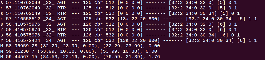
trace 文件的各项含义:
| 序号 | 数据名称 | 数据内容 |
|---|---|---|
| 1 | 事件类型 | s(发送事件) r(接收事件) d(丢弃事件) f(转发事件) |
| 2 | 时间 | 产生的时间 |
| 3 | 处理该事件的节点 | ID |
| 4 | Trace 种类 | RTR:路由器 / AGT:代理 / MAC:MAC 层 |
| 5:6 | 分隔符 | - |
| 7 | 分组 | ID |
| 8 | 分组类型 | - |
| 9 | 分组大小 | - |
| 10 | 发送节点在无线信道上发送该分组所期望的时间值 | - |
| 11 | 接收节点的 MAC 地址 | MAC 地址 |
| 12 | 发送节点的 MAC 地址 | MAC 地址 |
| 13 | MAC 层封装的分组类型 | 0x800:IP 分组 / 0x806:ARP 分组 |
| 14:16 | 分隔符 | - |
| 17 | 分组发送的源 IP 地址 | 节点号.端口号 |
| 18 | 分组发送的目的 IP 地址 | 节点号.端口号 |
| 19 | 分组的 TTL 值 | TTL |
| 20 | 源节点到目的节点的跳数 | 跳数 |
- 分析数据
我们需要对 Trace 文件进行查看,重点应该关注在分组类型为 AODV 的数据上,如下截图:
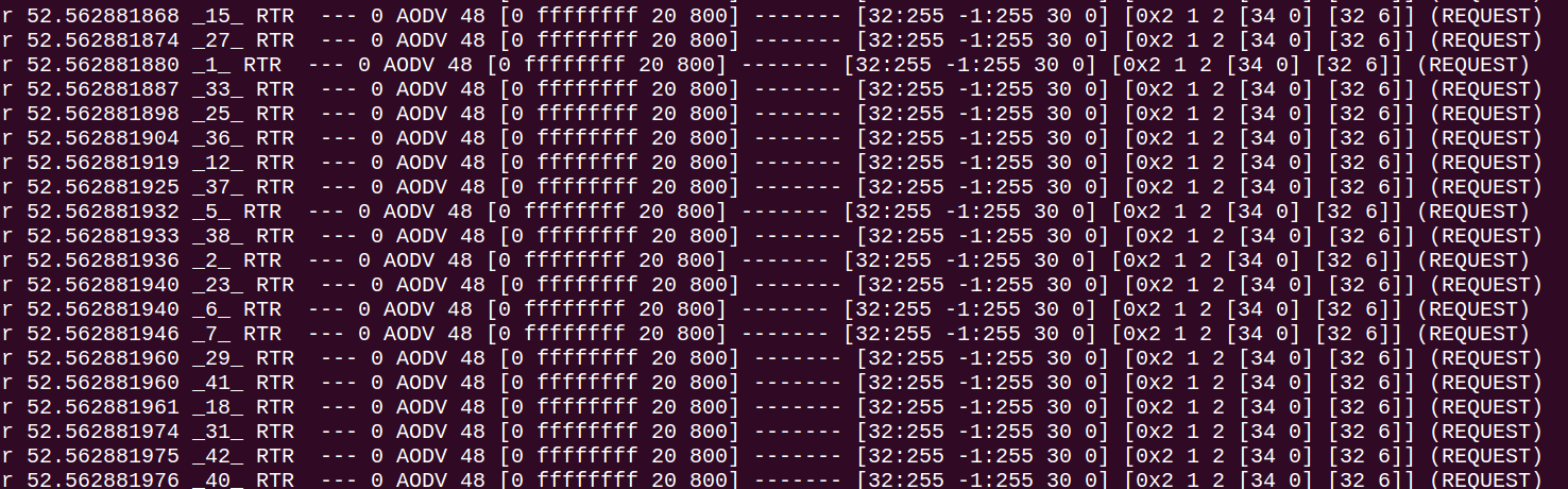
对某一个固定分组的消息进行追踪,可以通过 linux 下的 grep 正则匹配来识别,经过查看分析以及查阅网上的资料,可以看到 AODV 有如下特点:
- 使用目的序列号来避免路由环路,避免了无限计数的问题
- 网络具有可拓展性;
- 支持中间节点应答,能使源节点快速获得路由,有效减少了广播数;
- 快速响应活跃路径上断链;需要周期性地广播分组;
- 不活跃的路由在一定时间后会被删除。
五、实验心得与体会
首先想要说的是这个实验其实我投机取巧了,本来 adov.tcl 应该是一个蛮大的编写量的,但是想到实验三有写过极为类似的脚本就重用了之前的代码,着实减轻了不少的负担。
另一个方面,这个实验也让我对 trace 文件有了更深入的了解。在实验三中我只是依样画葫芦地使用 gawk 脚本对 trace 文件进行分析,在这个实验中我自己去理解并阅读了 trace 文件,对整个文件结构也就有了更深入的理解,对未来我更进一步地学习 ns-2 打了一个很好的基础。
同时,这个实验也让我了解到了 AODV 路由协议的特点,通过距离矢量路由协议,建立起了虚电路,从而搭建起整个路由网络,虽然开始建立的时候会花一些时间,但是后面效率很高,正如我之前说的一样,网络协议的追求是平衡性的越来越完善。也正是这个实验,给了我一个机会去温习并回忆计算机网络当时学习到的知识,感觉收益颇丰。
黑洞攻击实验
一、实验目的
通过本实验,掌握主动黑洞、被动攻击的原理与实现方法。
二、实验原理
- 被动型黑洞:
我们将一般意义上的黑洞节点称为被动型黑洞,这种攻击者转发经过自己的路由报文,但丢弃所有的数据报文,从而达到路由欺骗的目的。由于没有向网络注入虚假报文,仅仅对网络拓扑进行攻击,因此,这种在其它文献中经常提到的黑洞攻击是一种被动的路由扰乱型攻击。
- 主动型黑洞:
相对应地,我们定义了主动型黑洞,这是一种“改良”的黑洞节点,在被动黑洞的基础上,冒充目的结点,提前回复 RREQ 报文,对外界宣称自己就是目的节点,以达到“主动出击”的目的,从而吸引更多的数据包。因此,这种攻击属于主动的路由扰乱型攻击。
三、实验内容
因为主动型黑洞是在被动黑洞的基础上构造出来的,于是我决定实现主动型黑洞,并自己构建出一个场景证明黑洞的成功构建。
四、实验步骤及测试结果
- NS-2 源码修改:
我主要对 ns-2.35/aodv/aodv.cc 中的文件进行了修改
首先加入对攻击节点的判断,通过引入一个 hacker 字段定义一个黑洞攻击节点:
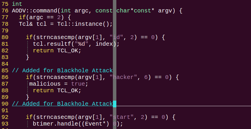
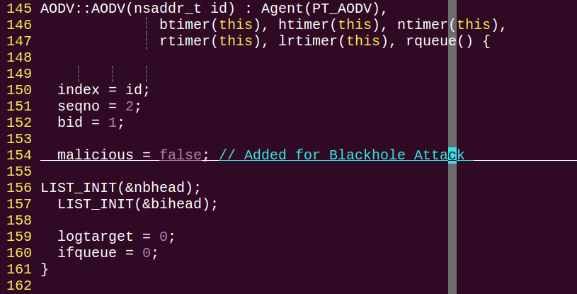
接下来在 AODV 的构造函数中加入一个 malicious 变量标志恶意报文:
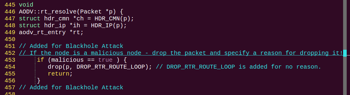
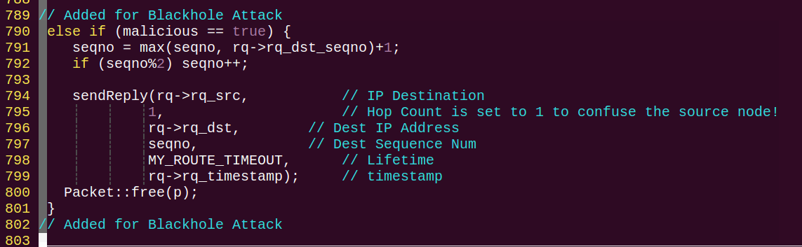
在 ADOV::rt_resolve 中,对黑洞攻击的恶意报文进行处理丢弃:
在 ADOV::recvRequest 中对恶意报文的源头进行混淆:
最后,更新 aodv.h:

这样一来,我们就实现了对一个黑洞节点的定义和黑洞报文的实现,接下来我们需要完善一个 balckhole.tcl 去对攻击场景进行模拟:
#===================================# Simulation parameters setup#===================================set val(chan) Channel/WirelessChannel ;# channel typeset val(prop) Propagation/TwoRayGround ;# radio-propagation modelset val(netif) Phy/WirelessPhy ;# network interface typeset val(mac) Mac/802_11 ;# MAC typeset val(ifq) Queue/DropTail/PriQueue ;# interface queue typeset val(ll) LL ;# link layer typeset val(ant) Antenna/OmniAntenna ;# antenna modelset val(ifqlen) 50 ;# max packet in ifqset val(nn) 7 ;# number of mobilenodesset val(rp) AODV ;# routing protocolset val(x) 800 ;# X dimension of topographyset val(y) 541 ;# Y dimension of topographyset val(stop) 100.0 ;# time of simulation end#===================================# Initialization#===================================#Create a ns simulatorset ns [new Simulator]#Setup topography objectset topo [new Topography]$topo load_flatgrid $val(x) $val(y)create-god $val(nn)#Open the NS trace fileset tracefile [open blackhole.tr w]$ns trace-all $tracefile#Open the NAM trace fileset namfile [open blackhole.nam w]$ns namtrace-all $namfile$ns namtrace-all-wireless $namfile $val(x) $val(y)set chan [new $val(chan)];#Create wireless channel#===================================# Mobile node parameter setup#===================================$ns node-config -adhocRouting $val(rp) \-llType $val(ll) \-macType $val(mac) \-ifqType $val(ifq) \-ifqLen $val(ifqlen) \-antType $val(ant) \-propType $val(prop) \-phyType $val(netif) \-channel $chan \-topoInstance $topo \-agentTrace ON \-routerTrace ON \-macTrace OFF \-movementTrace ON#===================================# Nodes Definition#===================================#Create 7 nodesset n0 [$ns node]$n0 set X_ 99$n0 set Y_ 299$n0 set Z_ 0.0$ns initial_node_pos $n0 20set n1 [$ns node]$n1 set X_ 299$n1 set Y_ 297$n1 set Z_ 0.0$ns initial_node_pos $n1 20set n2 [$ns node]$n2 set X_ 499$n2 set Y_ 298$n2 set Z_ 0.0$ns initial_node_pos $n2 20set n3 [$ns node]$n3 set X_ 700$n3 set Y_ 299$n3 set Z_ 0.0$ns initial_node_pos $n3 20set n4 [$ns node]$n4 set X_ 199$n4 set Y_ 350$n4 set Z_ 0.0$ns initial_node_pos $n4 20set n5 [$ns node]$n5 set X_ 599$n5 set Y_ 350$n5 set Z_ 0.0$ns initial_node_pos $n5 20set n6 [$ns node]$n6 set X_ 600$n6 set Y_ 200$n6 set Z_ 0.0$ns initial_node_pos $n6 20# Node 5 is given RED Color and a label- indicating it is a Blackhole Attacker$n5 color red$ns at 0.0 "$n5 color red"$ns at 0.0 "$n5 label Attacker"# Node 0 is given GREEN Color and a label - acts as a Source Node$n0 color green$ns at 0.0 "$n0 color green"$ns at 0.0 "$n0 label Source"# Node 3 is given BLUE Color and a label- acts as a Destination Node$n3 color blue$ns at 0.0 "$n3 color blue"$ns at 0.0 "$n3 label Destination"#===================================# Set node 5 as attacker#===================================$ns at 0.0 "[$n5 set ragent_] hacker"#===================================# Agents Definition#===================================#Setup a UDP connectionset udp0 [new Agent/UDP]$ns attach-agent $n0 $udp0set null1 [new Agent/Null]$ns attach-agent $n3 $null1$ns connect $udp0 $null1$udp0 set packetSize_ 1500#===================================# Applications Definition#===================================#Setup a CBR Application over UDP connectionset cbr0 [new Application/Traffic/CBR]$cbr0 attach-agent $udp0$cbr0 set packetSize_ 1000$cbr0 set rate_ 0.1Mb$cbr0 set random_ null$ns at 1.0 "$cbr0 start"$ns at 100.0 "$cbr0 stop"#===================================# Termination#===================================#Define a 'finish' procedureproc finish {} {global ns tracefile namfile$ns flush-traceclose $tracefileclose $namfileexec nam blackhole.nam &exit 0}for {set i 0} {$i < $val(nn) } { incr i } {$ns at $val(stop) "\$n$i reset"}$ns at $val(stop) "$ns nam-end-wireless $val(stop)"$ns at $val(stop) "finish"$ns at $val(stop) "puts \"done\" ; $ns halt"$ns run
颜色非常好定义,通过 color 就可以实现了,然后我的实验思路是:将 116 行的将 n5 定义为 hacker 的语句注释掉,就可以得到一个正常的网络,随后我们可以在将注释取消,得到一个带有黑洞节点的攻击网络,通过比对两个网络的模拟图像,同时分析 trace 文件我们可以得到相关的数据,并得出结论。这样我们就需要一个合适的 gawk 脚本:
BEGIN {sendLine = 0;recvLine = 0;fowardLine = 0;}$0 ~/^s.* AGT/ {sendLine ++ ;}$0 ~/^r.* AGT/ {recvLine ++ ;}$0 ~/^f.* RTR/ {fowardLine ++ ;}END {printf "cbr s:%d r:%d, r/s Ratio:%.4f, f:%d \n", sendLine, recvLine, (recvLine/sendLine),fowardLine;}
同样,我们也可以通过设置发包速率来横向比对各种数据。
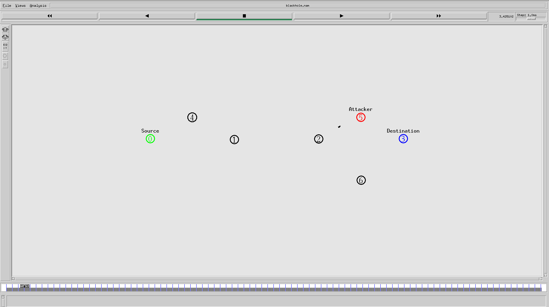
正常情况下的 nam 图像:
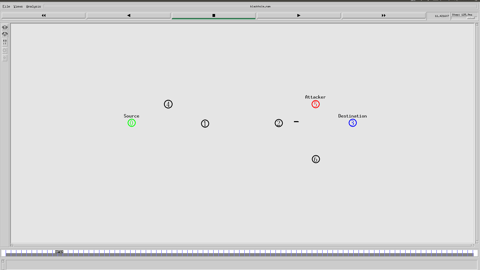
有黑洞节点的 nam 图像:
可以看到,明显黑洞节点吸引了报文,一下是两个 trace 对比情况的截图:
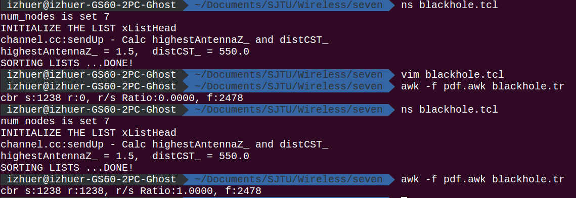
有黑洞节点的丢包率是是百分之百,可见攻击效果多明显。
五、实验心得与体会
在这个实验中,我并没有按照实验的要求去绘制攻击者数量和丢包率的关系图,主要原因在于当我把大量的节点放置在网络中时,我发现我的 ns 出现了段错误,这个问题一直没有解决,个人猜测是因为对黑洞信息的处理不得当的原因,但是不得不说的是,这个黑洞实验着实锻炼了我不少。不像之前的虫洞试验,深入 ns-2 源码中对错误进行了很久的分析也没有找到失败的原因。这次黑洞实验,可能是因为有了虫洞实验的失败教训,我着实效率很高。深入思考了一下黑洞试验和虫洞实验对代码修改的难度差异,我觉得可能下面的主要愿意造成的:
- 黑洞实验中不需要对接收和发送同时处理,这样一来报文错误处理的可能性就大大减少了
- 而虫洞实验需要对接收和发送同时处理,而且代码中的
send_up和send_down不是简单的发出接收的函数,而是在网络模型的上下层传递的过程,这个就导致了牵一发动全身,使得冲动实验中有很多很多需要修改的部分。
另外的一点是,除了虫洞攻击实验,黑洞实验是我所有实验中难度最大的实验,我从一次次失败,一次次克服困难的过程中也学到了很多除了课程之外的更多的东西。谢谢老师和助教给我这样一个机会去提升自我。
