Computational Physics Homework 12 of Mobingbihzen

computational_physics homework

Name： 余康
Student Number: 2014301020117

1. Abstract

EXERCISE5.7. Write two programs to solve the capacitor problem of Figure 5.6 and 5.7, one using the Jacobi method and one using the SOR algorithm. For a fixed accuracy(as set by the convergence test) compare the number of iterations, $N_{iter}$, that each algorithm requires as a function of the number of grid elements, $L$. Show that for the Jocabi method $N_{iter} \sim L ^ 2$, while with SOR $N_{iter} \sim L$.

2. Background

2.1 Relaxation (iterative method)

In numerical mathematics, relaxation methods are iterative methods for solving systems of equations, including nonlinear systems.

Relaxation methods were developed for solving large sparse linear systems, which arose as finite-difference discretizations of differential equations. They are also used for the solution of linear equations for linear least-squares problems and also for systems of linear inequalities, such as those arising in linear programming. They have also been developed for solving nonlinear systems of equations.

Relaxation methods are important especially in the solution of linear systems used to model elliptic partial differential equations, such as Laplace's equation and its generalization, Poisson's equation. These equations describe boundary-value problems, in which the solution-function's values are specified on boundary of a domain; the problem is to compute a solution also on its interior. Relaxation methods are used to solve the linear equations resulting from a discretization of the differential equation, for example by finite differences.

These iterative methods of relaxation should not be confused with "relaxations" in mathematical optimization, which approximate a difficult problem by a simpler problem, whose "relaxed" solution provides information about the solution of the original problem.

2.2 Jacobi Method

In numerical linear algebra, the Jacobi method (or Jacobi iterative method) is an algorithm for determining the solutions of a diagonally dominant system of linear equations. Each diagonal element is solved for, and an approximate value is plugged in. The process is then iterated until it converges. This algorithm is a stripped-down version of the Jacobi transformation method of matrix diagonalization. The method is named after Carl Gustav Jacob Jacobi.

2.3 SOR Algorithm

In numerical linear algebra, the method of successive over-relaxation (SOR) is a variant of the Gauss–Seidel method for solving a linear system of equations, resulting in faster convergence. A similar method can be used for any slowly converging iterative process.

It was devised simultaneously by David M. Young, Jr. and by Stanley P. Frankel in 1950 for the purpose of automatically solving linear systems on digital computers. Over-relaxation methods had been used before the work of Young and Frankel. An example is the method of Lewis Fry Richardson, and the methods developed by R. V. Southwell. However, these methods were designed for computation by human calculators, and they required some expertise to ensure convergence to the solution which made them inapplicable for programming on digital computers. These aspects are discussed in the thesis of David M. Young, Jr.

3. Main

3.1 Formulation and Algorithm

Here what we need to deal with is the Laplace's equation:

$$\begin{equation} \frac{\partial ^ 2V}{\partial x ^ 2} + \frac{\partial ^ 2V}{\partial y ^ 2} + \frac{\partial ^ 2V}{\partial z ^ 2} = 0. \end{equation}$$
The numerical solution to this equation is :
$$\begin{equation} V(i, j, k) = \frac{1}{6}[V(i + 1, j, k) + V(i - 1, j, k) + V(i, j + 1, k)\\ + V(i, j - 1, k) + V(i, j, k + 1) + V(i, j, k - 1)], \end{equation}$$

Assuming the system we investigate is infinite along $\pm z$, thus our problem is transferred into a two-dimensional one, with the solution reducing to:

$$\begin{equation} V(i, j, k) = \frac{1}{4}[V(i + 1, j, k) + V(i - 1, j, k) + V(i, j + 1, k) + V(i, j - 1, k)]. \end{equation}$$

3.1.1 Jacobi Method

Mathematically the Jacobi method can be expressed as:

$$\begin{equation} V_{new}(i, j) = \frac{1}{4} [V_{old}(i + 1, j) + V_{old}(i -1, j) + V_{old}(i, j + 1) + V_{old}(i, J -1)], \end{equation}$$

where for simplicity we have assumed a two-dimensional problem and taken the grid size to be the same along $x$ and $y$.

3.1.2 Gauss-Seidel Method

The Gauss-Seidel method differs in that it uses the new values as they become available. If you move along each column $(i)$ from small $i$ to large $i$, beginning with the top row (small $j$), the Gauss-Seidel method can be written as

$$\begin{equation} V_{new}(i, j) = \frac{1}{4}[V_{old}(i + 1, j) + V_{new}(i -1, j) + V_{old}(i, J + 1) + V_{new}(i, j - 1)]. \end{equation}$$

3.1.3 SOR Algorithm

Let $V ^ {*}(i, j)$ be the new value of the potential calculated using the Gauss-Seidel method. The change recommended by the Gauss-Seidel method is:

$$\begin{equation} \Delta V(i, j) = V ^ {*}(i, j) - V_{old}(i, j), \end{equation}$$
To speed up convergence we will change the potential by a larger amount calculated according to:
$$\begin{equation} V_{new}(i, j) = \alpha \Delta V(i, j) + V_{old}(i, j), \end{equation}$$
where $\alpha$ is a factor that measures how much we "over-relax." For a probelm on a two-dimensional square grid like the ones we have considered and with fixed-value boundary conditons (called Dirichlet boundary conditions) on all four sides, the best choice for $\alpha$ is:
$$\begin{equation} \alpha \approx \frac{2}{1 + \pi/L}. \end{equation}$$

3.2 Results

3.2.1 Initialization

The first routine is to set the initial values for $V(i, j)$ (satisfying the boundary conditions at the same time.)

0.00 0.00 0.00 0.00 0.00 0.00 0.00 0.00 0.00 0.00 0.00 0.00 0.00 0.00 0.00 0.00 0.00 0.00 0.00 0.00
0.00 0.00 0.00 0.00 0.00 0.00 0.00 0.00 0.00 0.00 0.00 0.00 0.00 0.00 0.00 0.00 0.00 0.00 0.00 0.00
0.00 0.00 0.00 0.00 0.00 0.00 0.00 0.00 0.00 0.00 0.00 0.00 0.00 0.00 0.00 0.00 0.00 0.00 0.00 0.00
0.00 0.00 0.00 0.00 0.00 0.00 0.00 0.00 0.00 0.00 0.00 0.00 0.00 0.00 0.00 0.00 0.00 0.00 0.00 0.00
0.00 0.00 0.00 0.00 0.00 0.00 0.00 0.00 0.00 0.00 0.00 0.00 0.00 0.00 0.00 0.00 0.00 0.00 0.00 0.00
0.00 0.00 0.00 0.00 0.00 0.00 0.00 0.00 0.00 0.00 0.00 0.00 0.00 0.00 0.00 0.00 0.00 0.00 0.00 0.00
0.00 0.00 0.00 0.00 0.00 0.00 1.00 0.00 0.00 0.00 0.00 0.00 0.00 -1.00 0.00 0.00 0.00 0.00 0.00 0.00
0.00 0.00 0.00 0.00 0.00 0.00 1.00 0.00 0.00 0.00 0.00 0.00 0.00 -1.00 0.00 0.00 0.00 0.00 0.00 0.00
0.00 0.00 0.00 0.00 0.00 0.00 1.00 0.00 0.00 0.00 0.00 0.00 0.00 -1.00 0.00 0.00 0.00 0.00 0.00 0.00
0.00 0.00 0.00 0.00 0.00 0.00 1.00 0.00 0.00 0.00 0.00 0.00 0.00 -1.00 0.00 0.00 0.00 0.00 0.00 0.00
0.00 0.00 0.00 0.00 0.00 0.00 1.00 0.00 0.00 0.00 0.00 0.00 0.00 -1.00 0.00 0.00 0.00 0.00 0.00 0.00
0.00 0.00 0.00 0.00 0.00 0.00 1.00 0.00 0.00 0.00 0.00 0.00 0.00 -1.00 0.00 0.00 0.00 0.00 0.00 0.00
0.00 0.00 0.00 0.00 0.00 0.00 1.00 0.00 0.00 0.00 0.00 0.00 0.00 -1.00 0.00 0.00 0.00 0.00 0.00 0.00
0.00 0.00 0.00 0.00 0.00 0.00 1.00 0.00 0.00 0.00 0.00 0.00 0.00 -1.00 0.00 0.00 0.00 0.00 0.00 0.00
0.00 0.00 0.00 0.00 0.00 0.00 0.00 0.00 0.00 0.00 0.00 0.00 0.00 0.00 0.00 0.00 0.00 0.00 0.00 0.00
0.00 0.00 0.00 0.00 0.00 0.00 0.00 0.00 0.00 0.00 0.00 0.00 0.00 0.00 0.00 0.00 0.00 0.00 0.00 0.00
0.00 0.00 0.00 0.00 0.00 0.00 0.00 0.00 0.00 0.00 0.00 0.00 0.00 0.00 0.00 0.00 0.00 0.00 0.00 0.00
0.00 0.00 0.00 0.00 0.00 0.00 0.00 0.00 0.00 0.00 0.00 0.00 0.00 0.00 0.00 0.00 0.00 0.00 0.00 0.00
0.00 0.00 0.00 0.00 0.00 0.00 0.00 0.00 0.00 0.00 0.00 0.00 0.00 0.00 0.00 0.00 0.00 0.00 0.00 0.00
0.00 0.00 0.00 0.00 0.00 0.00 0.00 0.00 0.00 0.00 0.00 0.00 0.00 0.00 0.00 0.00 0.00 0.00 0.00 0.00

What we need to do is to save it in a txt file like this:

Figure 1: This matrix discribe the boundary conditions we investigate in a 20 $\times$ 20 lattice.

Then comes the question that how we can read and write our boundary conditions files in our python program. Here it is:

def initialization(self,initial_file):
    itxt= open(initial_file)
    self.lattice_in = []
    self.lattice_out = []
    for lines in itxt.readlines():
        lines=lines.replace("\n","").split(",")    
        self.lattice_in.append(lines[0].split(" "))
        self.lattice_out.append(lines[0].split(" "))
    itxt.close()
    for i in range(len(self.lattice_in)):
        for j in range(len(self.lattice_in[i])):
            self.lattice_in[i][j] = float(self.lattice_in[i][j])
            self.lattice_out[i][j] = float(self.lattice_out[i][j])
    return 0

3.2.2 Results of the Jacobi method

†
* 5 $\times$ 5 lattice

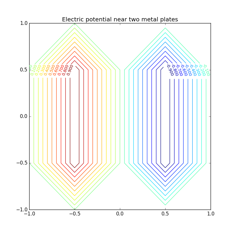
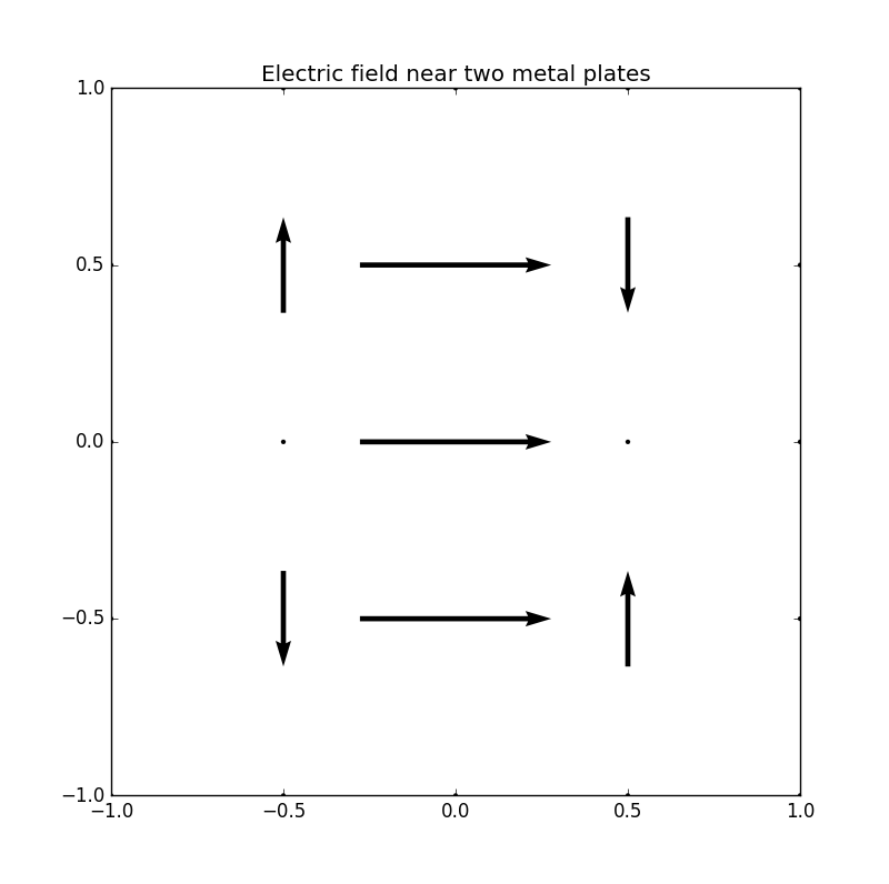
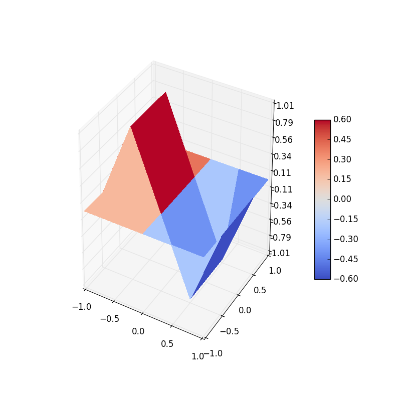
Figure 2: Electric potential and field near two capacitor plates simulated by $5 \times 5$ lattice. Upper: equipotential† lines; middle: electric field; bottom: perspective plot of the potential.

• 8 $\times$ 8 lattice
  
  
  

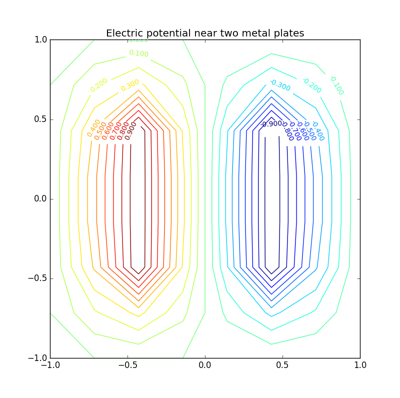
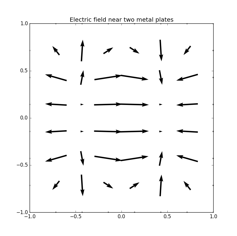
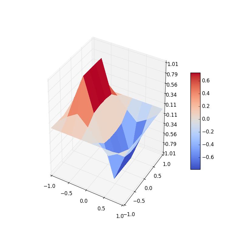
  Figure 3: Electric potential and field near two capacitor plates simulated by $8 \times 8$ lattice. Upper: equipotential lines; middle: electric field; bottom: perspective plot of the potential.

• 11 $\times$ 11 lattice
  
  
  

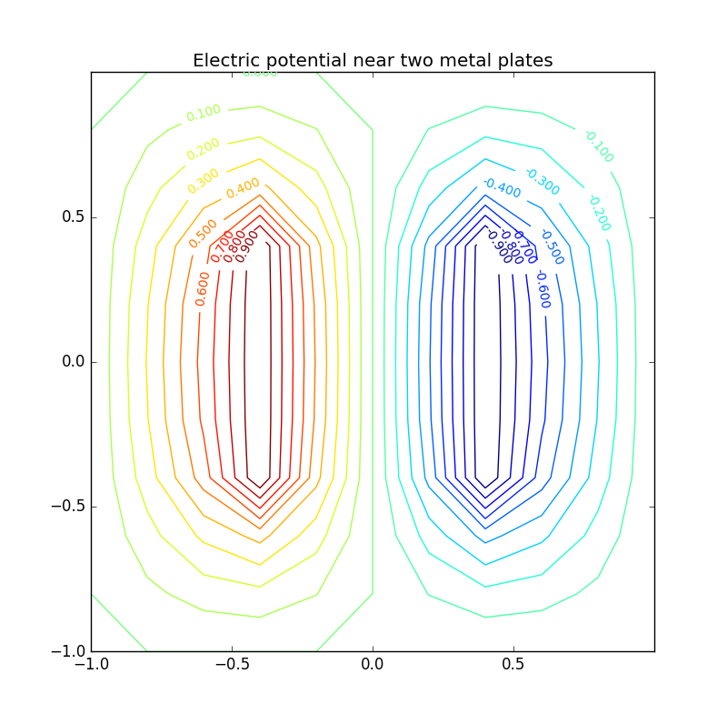
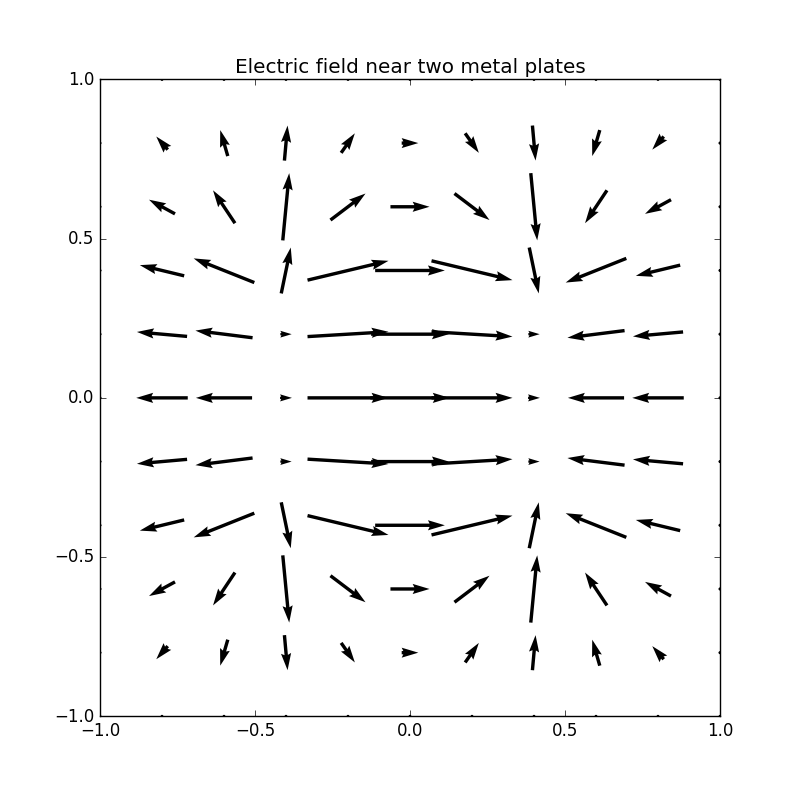
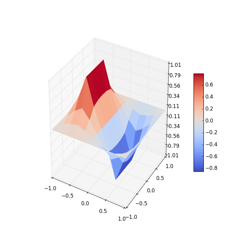
  Figure 4: Electric potential and field near two capacitor plates simulated by $11 \times 11$ lattice. Upper: equipotential lines; middle: electric field; bottom: perspective plot of the potential.

• 14 $\times$ 14 lattice
  
  
  

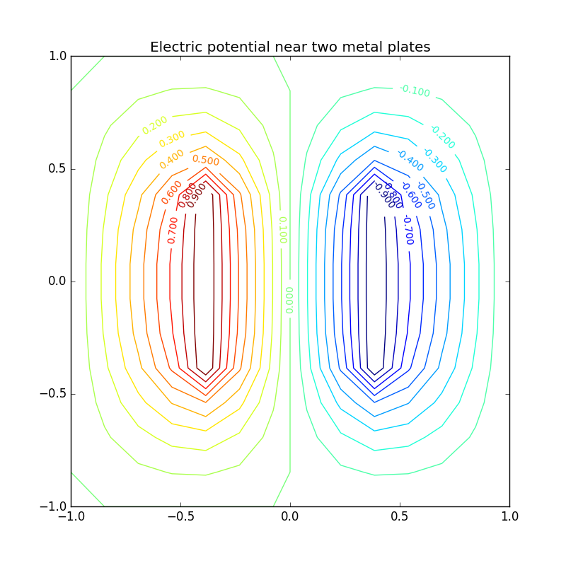
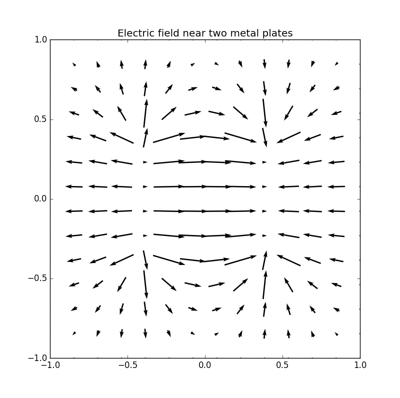
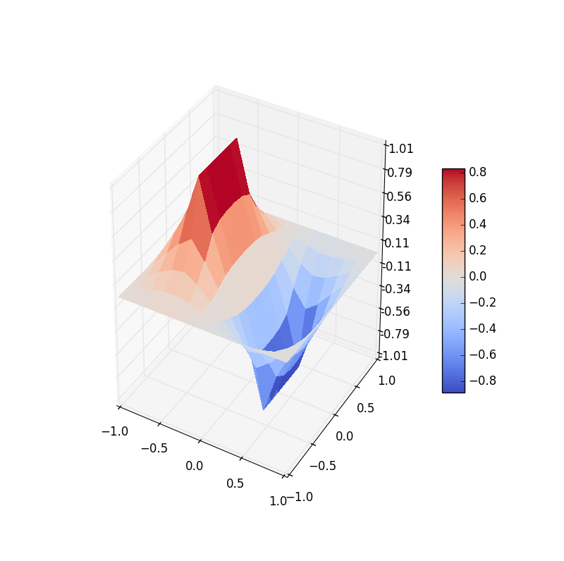
  Figure 5: Electric potential and field near two capacitor plates simulated by $14 \times 14$ lattice. Upper: equipotential lines; middle: electric field; bottom: perspective plot of the potential.

• 20 $\times$ 20 lattice
  
  
  

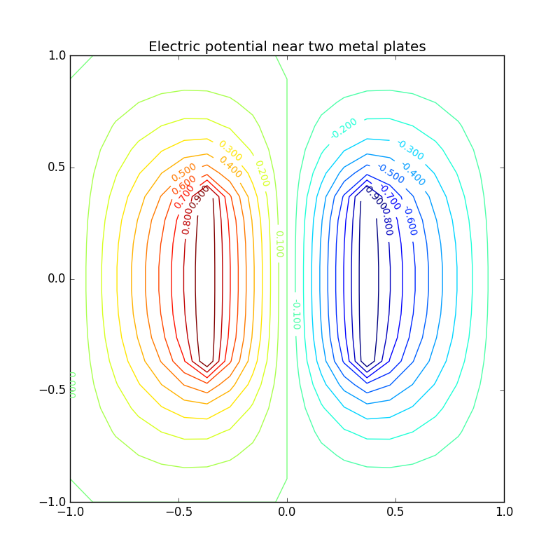
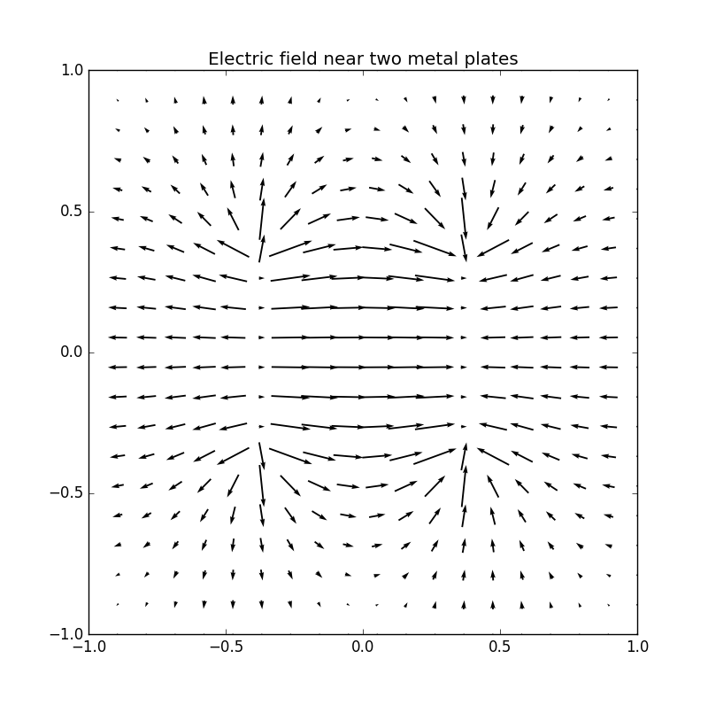
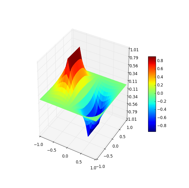
  Figure 6: Electric potential and field near two capacitor plates simulated by $20 \times 20$ lattice. Upper: equipotential lines; middle: electric field; bottom: perspective plot of the potential.

• 23 $\times$ 23 lattice
  
  
  

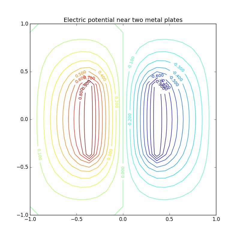
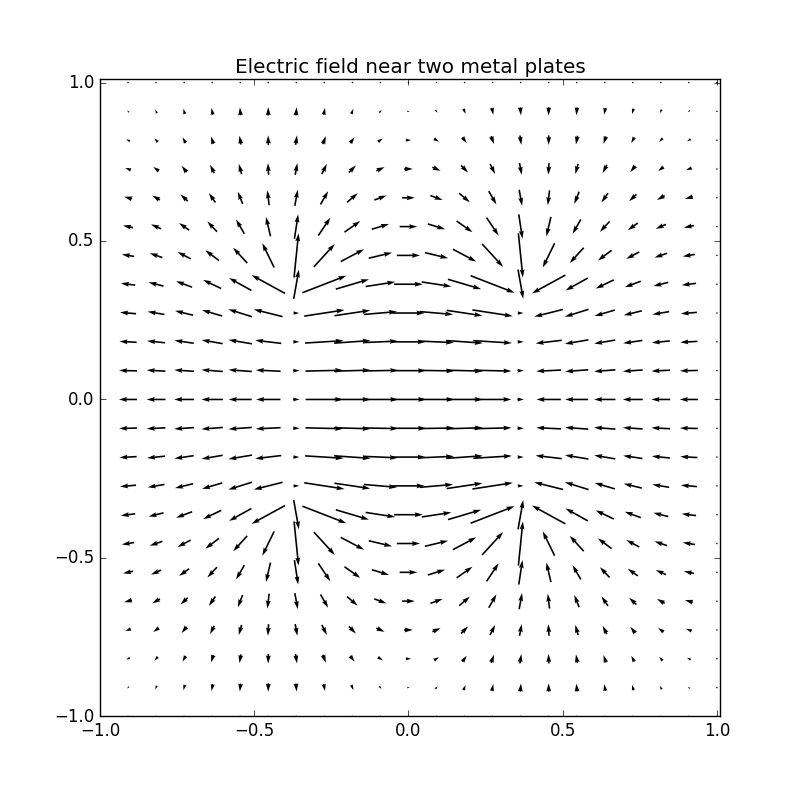
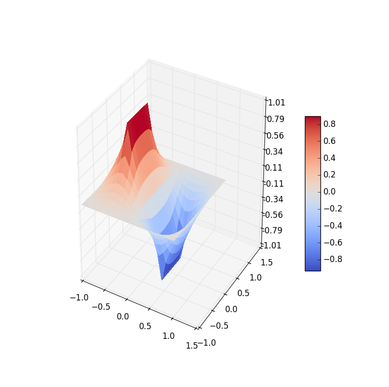
  Figure 7: Electric potential and field near two capacitor plates simulated by $23 \times 23$ lattice. Upper: equipotential lines; middle: electric field; bottom: perspective plot of the potential.

• 26 $\times$ 26 lattice
  
  
  

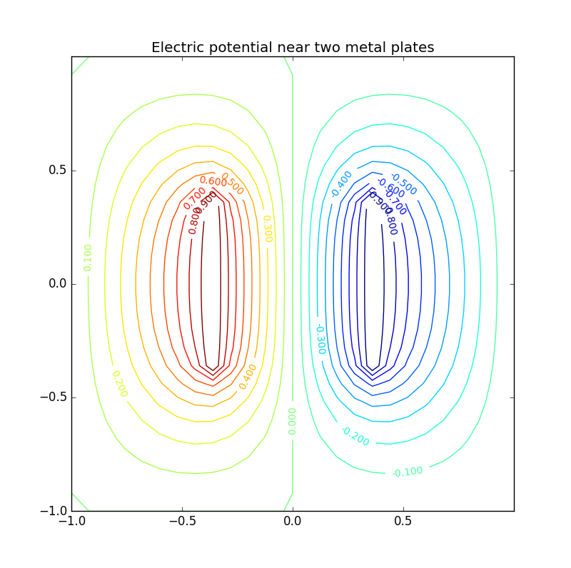
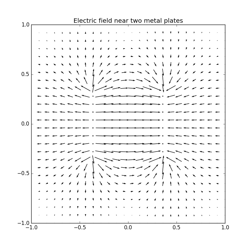
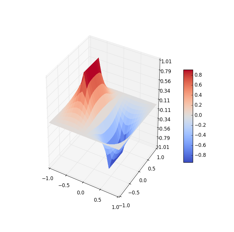
  Figure 7: Electric potential and field near two capacitor plates simulated by $26 \times 26$ lattice. Upper: equipotential lines; middle: electric field; bottom: perspective plot of the potential.

---

‡
Results of relationship between the convergence speed of Jacobi method and the number of grid elements
First of all, there is an example:

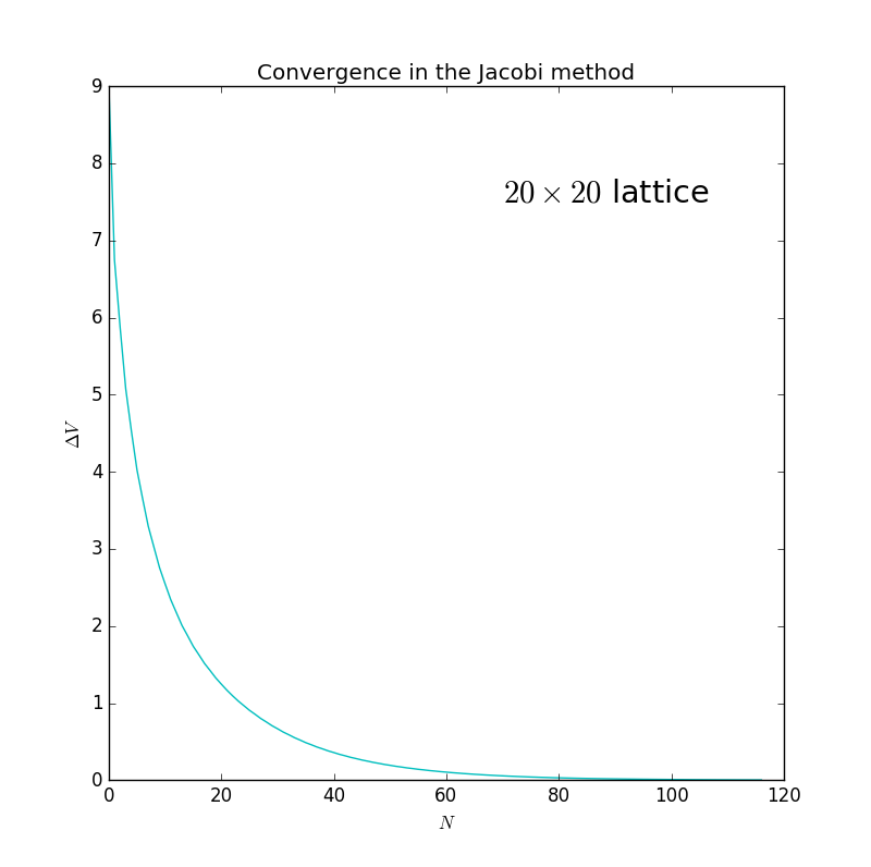
Figure 8: This is the convergence cituation when the number of elements $L = 20.$

There are all values of the number of iterations $N_{iter}$ and their corresponding number of grid elements $L$ in the Jacobi method.

$L$	$N_{iter}$
5	1
8	18
11	30
14	59
20	117
23	139
26	189

This is the plot of the sheet above:

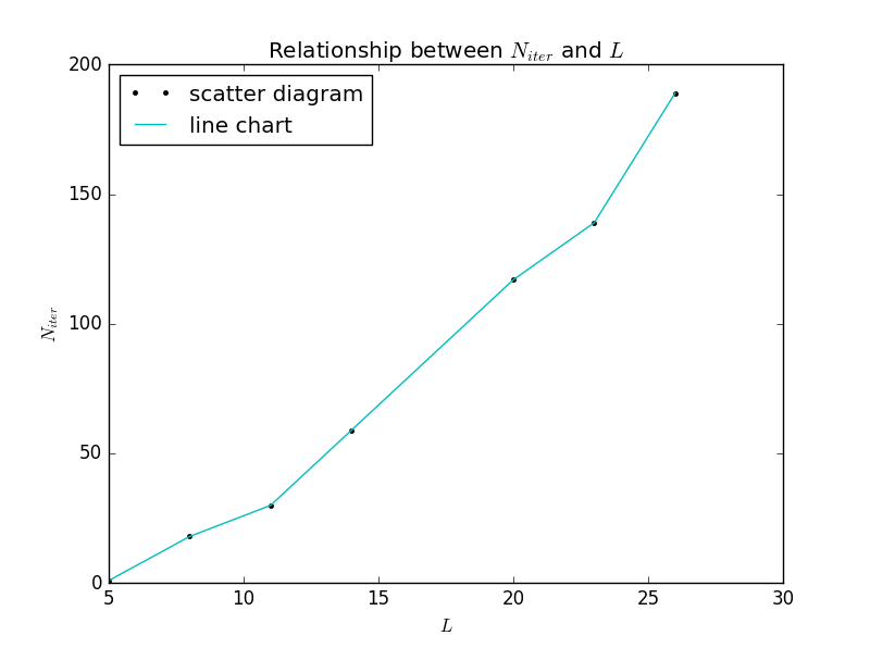
Figure 9: The relationship between $N_{iter}$ and $L$ in the Jacobi method.

And this is the fitting curve of Matlab:

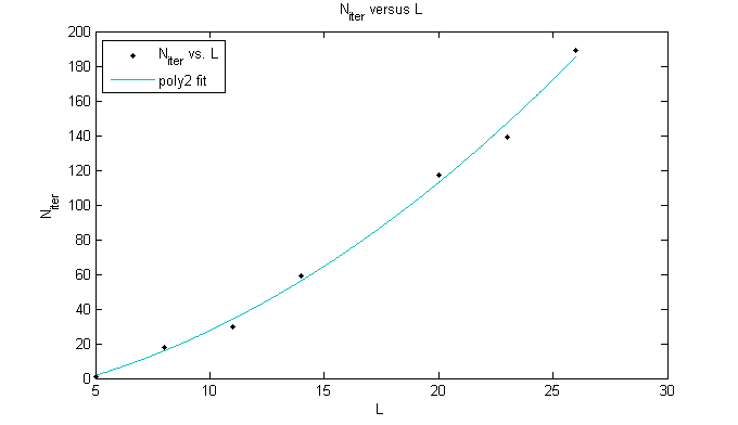
Figure 10: The Matlab fitting curve of $N_{iter}$ versus $L$ in the Jacobi method.

We can see that $N_{iter} \sim L ^ 2$ approximately.

---

3.2.3 Results of the SOR algorithm

†
Results of relationship between the convergence speed of SOR algorithm and the number of grid elements
First of all, there is an example:

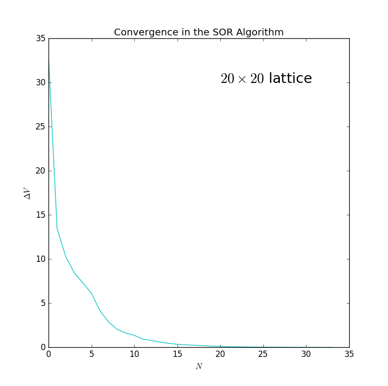
Figure 11: This is the convergence cituation when the number of elements $L = 20$ in the SOR algorithm.

There are all values of the number of iterations $N_{iter}$ and their corresponding number of grid elements $L$ in the SOR algorithm.

$L$	$N_{iter}$
5	1
8	14
11	19
14	24
20	34
23	39
26	44

This is the plot of the sheet above:

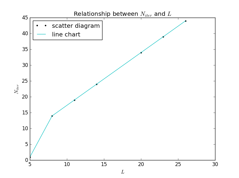
Figure 12: The relationship between $N_{iter}$ and $L$ in the SOR algorithm.

And this is the fitting curve of Matlab:

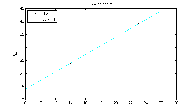
Figure 13: The Matlab fitting curve of $N_{iter}$ versus $L$ in the SOR algorithm (for accuracy I dropped out the first point which is far away from the almost perfect fitting stright line).

We can see that $N_{iter} \sim L$ approximately.

program code

---

4. conclusion

I have mentioned in the context:

• $N_{iter} \sim L ^ 2$ approximately

• $N_{iter} \sim L$ approximately

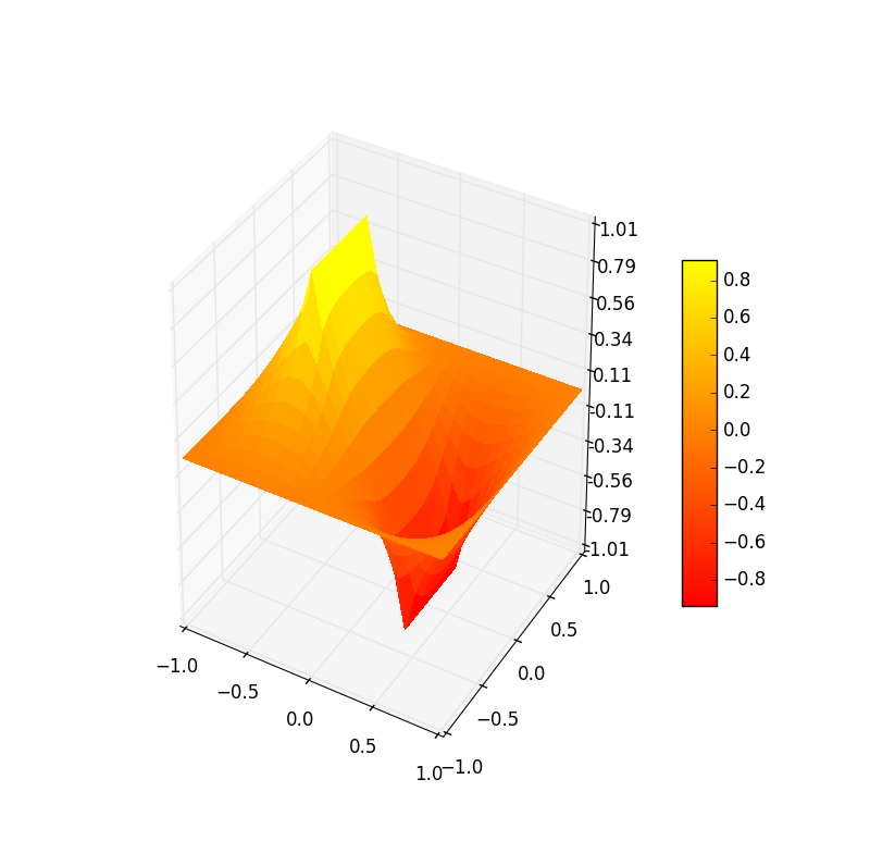
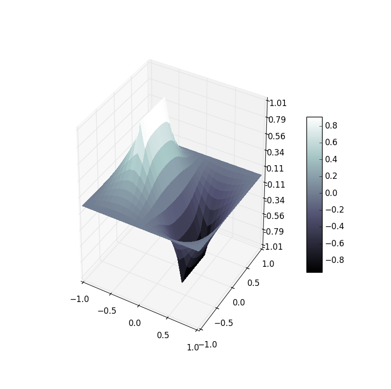
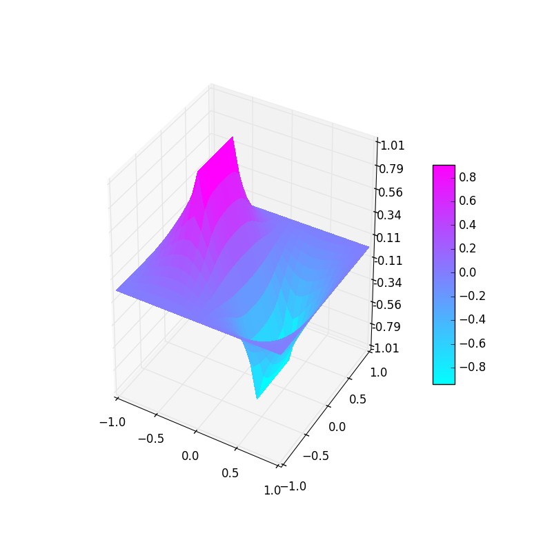
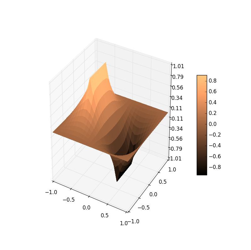
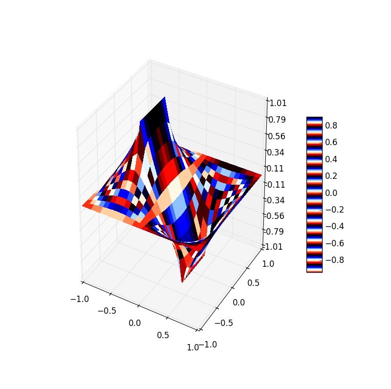
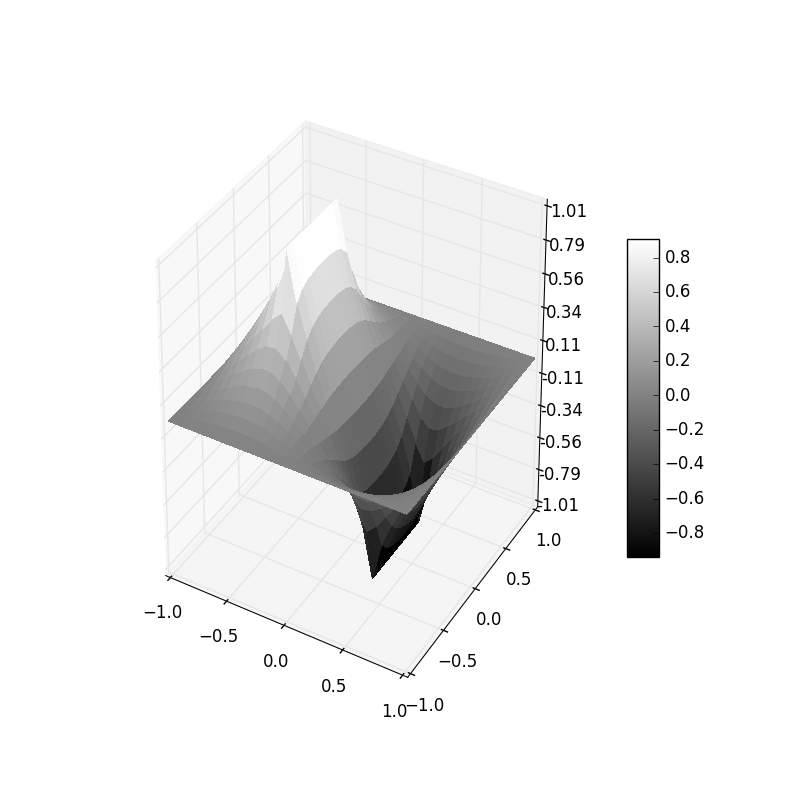
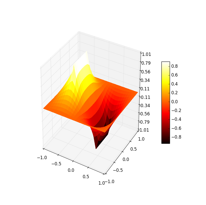
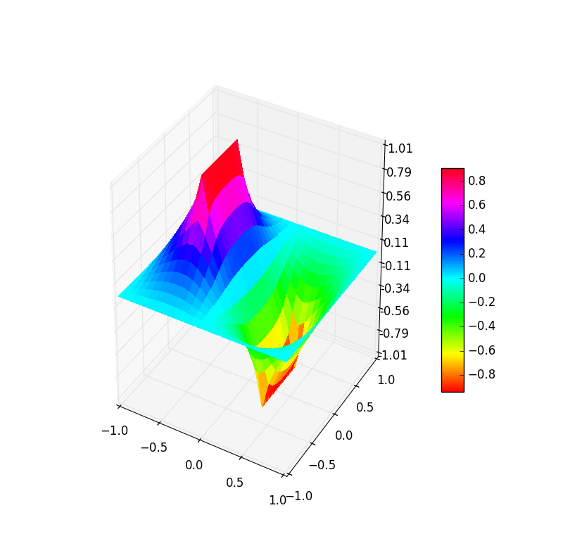
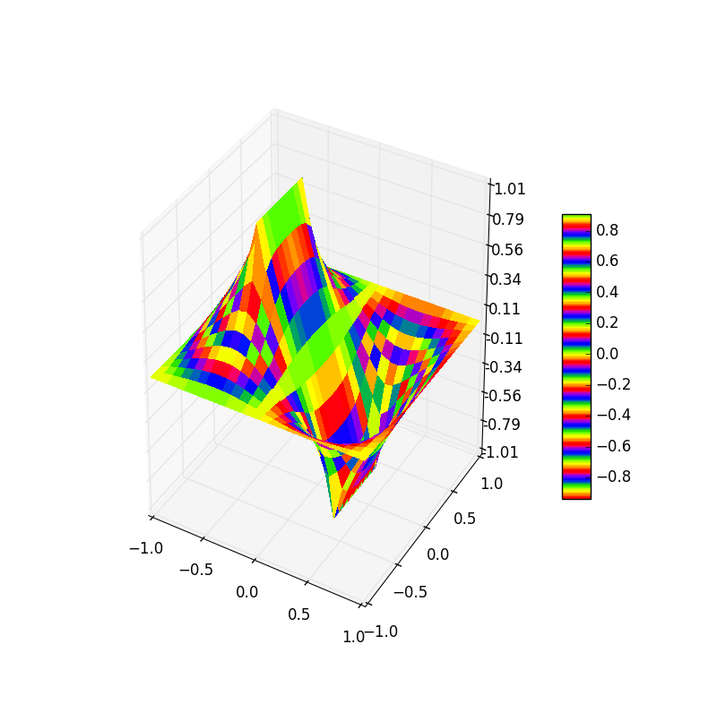
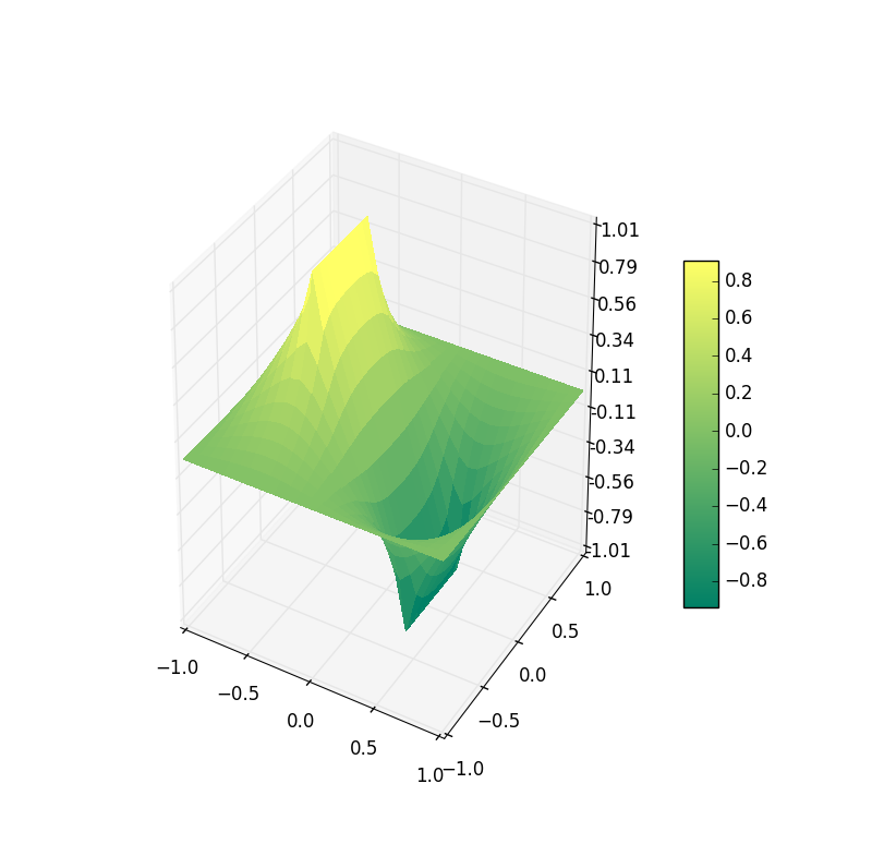
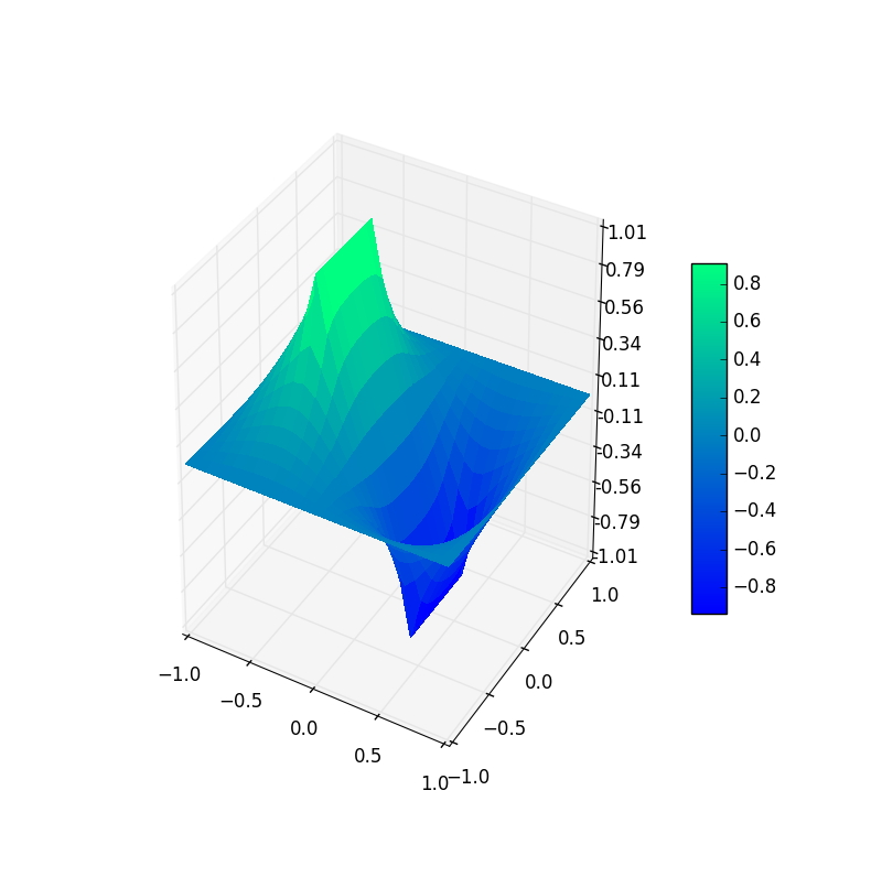
At last, I learned how to plot colorful 3D figures:

• jet
  

• autumn
  

• bone
  

• cool
  

• copper
  

• flag
  

• gray
  

• hot
  

• hsv
  

• prism
  

• spring
  

• summer
  

• winter
  

5. acknowledgement

• our devoted Prof. Cai
• Wikipedia
• Cheng Feng
• Ni Shijie