Molecular Dynamics Using GROMACS

Moleculle Dynamics GROMACS Simulation

Software: GROMACS: http://www.gromacs.org

Manual: http://www.gromacs.org/Documentation/Manual

Platform: Linux

Initial Protein Structure: cns1_model1.pdb

1 Check GROMACS

GROMACS location:

/usr/local/gromacs/bin/

Set environment variable:

export PATH=$PATH:/usr/local/gromacs/bin/
#test if environment works
gmx -version

Result:

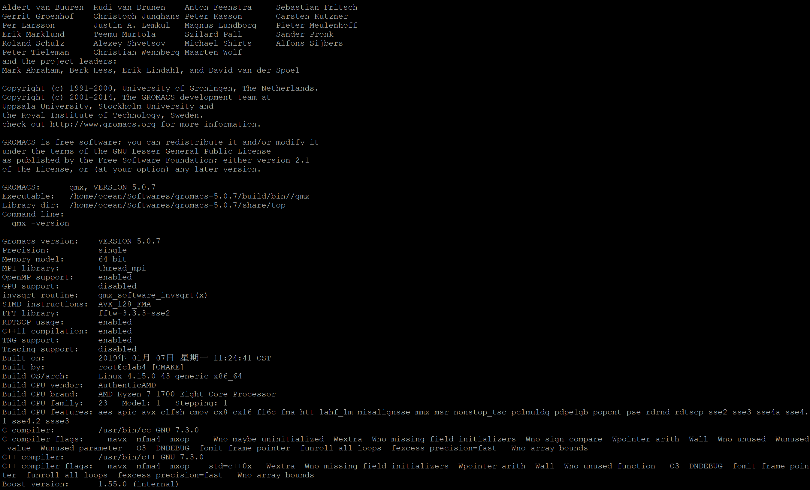
So, it works.

2 cns1_model1 MD Simulation

2.1 protein pdb file preprocessing

1 . Remove the crystal waters in the pdb file
Use grep to delete these lines very easily:

grep -v HOH cns1_model1.pdb > cns1_clean.pdb

2.3 Molecule Dynamics Simulation

1 . Transfer pdb to gmx format, which contains:

• The topology for the molecule.
• A position restraint file.
• A post-processed structure file.

gmx pdb2gmx -ignh -ff amber99sb-ildn -f cns1_clean.pdb -o cns1_clean.gro -p cns1_clean.top -water tip3p

• -ignh: Ignore all hydrogen atoms, because if H atoms are present, they must be in the named exactly how the force fields in GROMACS expect them to be. So dealing with H atoms can occasionally be a headache!
• -ff: We use Amber99SB-ILDN force field.
• -f: Specify the input file name
• -o: Specify the newly output GROMCAS file
• -p: Specify the newly ouput topology file, including the parameters of all atom-atom interactions.
• -water: Specify the mater model. We use TIP3P water model.

2 . Create the simulation box

We use editconf operation to create periodic simulation box.

gmx editconf -f cns1_clean.gro -o cns1_clean-PB.gro -bt cubic -d 1.2
#-bt dodecahedron (dodecahedron is probable better in other situations)

• -f: Input protein structure.
• -o: Output structure file with the simulation box information.
• -bt: Simulation box tyoe, default: rectangle box.
• -d: The minimum distance of the protein feom the X, Y, Z direction of the simulation box.

We use -bt option to create the rhombic dodecahedron, because its volume is ~71% of the cubic box of the same periodic distance, thus saving on the number of water molecules that need to be added to solvate the protein. -d option specifies the minimum distance of the molecule to the box margin, using nm as the unit. It specifies the size of the box. In theory, of the majority of the systems, -d can not be less than 0.9nm, so we use 1.2nm.

We can check the structure of the protein with the added box. We need to transfer the gro format to pdb format using editconf operation

For example, we can convert the file.gro to file.pdb

gmx editconf -f file.gro -o file.pdb

3 . Energy minimization of the protein molecule in vaccum

We should design the specific .mdp file to specify parameters.

em-vac-pme.mdp

; Definition delivered to preprocessor
define          = -DFLEXIBLE    ; Use flexible water model rather than rigid water model, thus steepest descent method will further minimize the energy
; Model type, Ending control, input control parameter
integrator      = steep         ; Algorithm (steep = steepest descent minimization)
emtol           = 500.0         ; Stop minimization when the maximum force < 1000.0 kJ/mol/nm
emstep          = 0.01          ; Minimization step size
nsteps          = 1000          ; Maximum number of (minimization) steps to perform
nstenergy       = 1             ; Energy writing frequency
energygrps      = System        ; Writing energy group
; Nearst list, interaction calculation parameter
nstlist         = 1             ; Frequency to update the neighbor list and long range forces
ns_type         = grid          ; Method to determine neighbor list (simple, grid)
coulombtype     = PME           ; Treatment of long range electrostatic interactions
rlist           = 1.0           ; 
rcoulomb        = 1.0           ; Short-range electrostatic cut-off
vdwtype         = cut-off       ; Method for calculating van der waals interaction
rvdw            = 1.0           ; Short-range Van der Waals cut-off
constraints     = none          ; Set the restriction of the model
pbc             = xyz           ; Periodic Boundary Conditions in all 3 dimensions

Gromacs pre-processor (grompp) can integrate all information including simulated parameter, molecular structure, molecular structure, acquired force field parameter into a single binary file (tpr file), so it requires only tpr file while running mdrun.

gmx grompp -f em-vac-pme.mdp -c cns1_clean-PB.gro -p cns1_clean.top -o cns1_em-vac.tpr

• -f option specifies the input parameter file
• -c option specifies the input structure file
• -p option soecifies the input topology file
• -o option specifies the output file which is used for mdrun

After that, we get file cns1_em-vac.tpr and parameter file mdout.mdp.

We use mdrun intruction to run the energy minimization

gmx mdrun -v -deffnm cns1_em-vac

• -deffnm specifies default file name
• -v shows the infomation of the simulation process

After 1001 steps, result is :

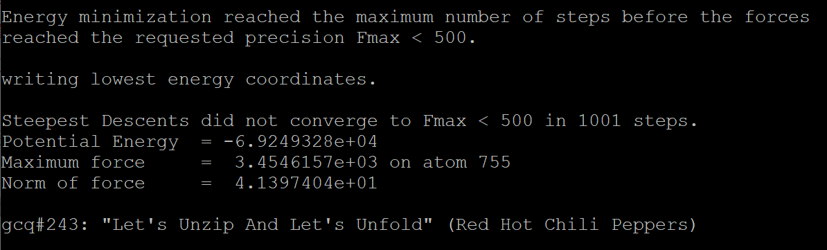
As a result, we get the record file cns1_em-vac.log, Binary full-precision trajectory cns1_em-vac.trr, Energy-minimized structure cns1_em-vac.gro.

If we only need the molecule dynamics simulation in vaccum, the above steps have got what we want, the .trr file, which can be depicted to movies using VMD software. However, if we need simulation in the solvent, water, for example, we have to go further.

4 . Infusing solvent and ion into the box and conduct energy minimization

We use gmx solvate to infuse the water into the box, simulating the solvation of the protein molecule.

gmx solvate -cp cns1_em-vac.gro -cs spc216.gro -p cns1_clean.top -o cns1-b4ion.gro

• -cp specifies the model of the simulating protein box
• -cs specifies the water model to be SPC water model used for infilling
• spc216 is the general 3-site water structure in GROMACS
• -p adjusts the topology file, adding the physical parameters of the corresponding water molecule
• -o specifies the output file after filling the water molecule

As a result, we get cns1-b4ion.gro.

Then we need to minimize the energy of the system, using another em-sol-pme.mdp file.

em-sol-pme.mdp

define          = -DFLEXIBLE
integrator      = steep
emtol           = 250.0
nsteps          = 5000
nstenergy       = 1
energygrps      = System
nstlist         = 1
ns_type         = grid
coulombtype     = PME
rlist           = 1.0
rcoulomb        = 1.0
rvdw            = 1.0
constraints     = none
pbc             = xyz

Likewise, we need to use grompp to process the .mdp file, after which we start to conduct mdrun.

gmx grompp -f em-sol-pme.mdp -c  cns1-b4ion.gro -p cns1_clean.top -o ion.tpr

The generated ion.tpr is the result, and the output message is as follows:

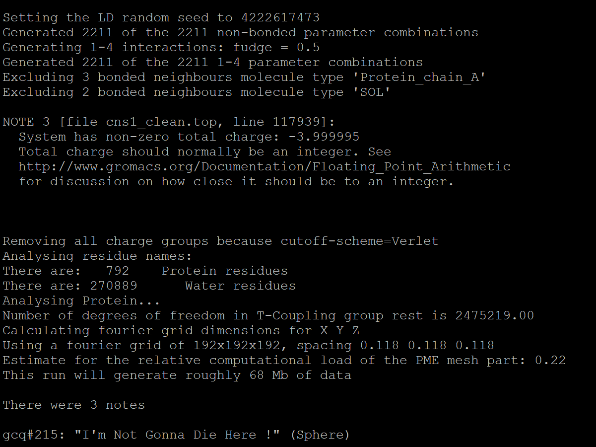
We can see from the message that the total charge is -3.999995. Since the total charge should be described in integers, there are around -4e charge.

Then, we need to add the ion into the system, using the ion.tpr file. The ion we add should neutralise the charge original in the system. Since we have -4e charge in the system, we need to add more negion than cation.

We use geion operation to replace some water molecules by ions.

gmx genion -s ion.tpr -o cns1-b4em.gro -neutral -conc 0.15 -p cns1_clean.top

• -neutral option garantee the whole charge in the system equals zero, and the system is neutralized.
• -conc option sets the required ion concentration (here we use 0.15M)
• -g option specifies the name of the output record file
• -norandom option set the ion according to the electric potential, not random (default). However, here we use random set, so we do not use this option

Aftering executing this operation, it appears a consecutive solvent molecule group. Here we choose 13(SOL). Typing Enter, the procudure will tell your your solvent molecules have been replaced by Cl ion.

Inorder to run energy minimization by mdrun, we have to use the grompp operation again.

gmx grompp -f em-sol-pme.mdp -c cns1-b4em.gro -p cns1_clean.top -o cns1_em-sol.tpr

Then, we run energy minimization:

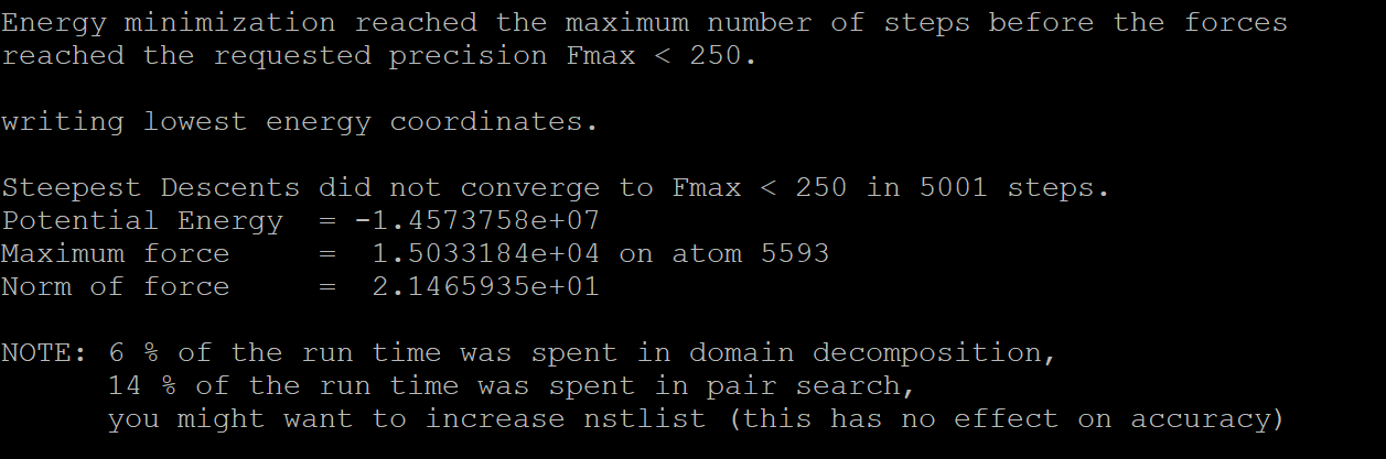
gmx mdrun -v -deffnm cns1_em-sol

We can see that after 5001 steps, it reaches convergence.

Note: genion uses NaCl in default. If users want any other negion and cation, they can use -pname (cation) and -nname (negion) to specify the name of the ions. Users can refer tothe ion.itp file to see how to call different ions

5 . Position-restricted pre-equalization simulation

We now need to construct position-restricted pre-equalization simulation, that is to say, we fix the position of the protein atoms and keep the solvent molecules moving, just like soaking the protein molecules into the water, enabling the further equilibration of the system.

We need to perform two stages of position-restricted pre-equalizations: 100ps NVT and 100ps NPT, with the temperature of 310 K, which is similar to the experiment room temperature. It is appropriate to simulate in 310 K, since it is similar to the body temperature.

Likewise, we need another .mdp file called nvt-pr-md.mdp file.

define                   = -DPOSRES ; Tell GROMACS run position restricted siulation
integrator               = md
dt                       = 0.002 ; step length, the unit of which is ps, here we use 2fs
nsteps                   = 50000 ; number of steps, the simulation time is nsteps*dt
; output control parameter
nstxout                  = 500   ; Writing frequency, nstxout=500 and dt=0.002, so it writes out every 1 ps
nstvout                  = 500   ; Velocity saving frequency
nstenergy                = 500   ; Energy saving frequency
nstlog                   = 500   ; log file output frequency
energygrps               = Protein Non-Protein
; 
nstlist                  = 5
ns_type                  = grid
pbc                      = xyz
rlist                    = 1.0
; 
coulombtype              = PME  
pme_order                = 4    
fourierspacing           = 0.16 
rcoulomb                 = 1.0  ; unit is nm
vdw-type                 = Cut-off
rvdw                     = 1.0
; 
tcoupl                   = v-rescale            
tc-grps                  = Protein  Non-Protein 
tau_t                    = 0.1      0.1         
ref_t                    = 300      300        
; 
DispCorr                 = EnerPres 
; 
pcoupl                   = no                    
; 
gen_vel                  = yes    
gen_temp                 = 300    
gen_seed                 = -1     
; 
constraints              = all-bonds    
continuation             = no           
constraint_algorithm     = lincs        
lincs_iter               = 1            
lincs_order              = 4            

Also, we need to use grommp and then mdrun again.

gmx grompp -f nvt-pr-md.mdp -c cns1_em-sol.gro -p cns1_clean.top -o cns1_nvt-pr.tpr
#gmx mdrun -deffnm cns1_nvt-pr

If mdrun requires so much time, users can use nohup to run the program background.

nohup gmx mdrun -deffnm cns1_nvt-pr &
#If you want to check the state of the program
tail -n 25 cns1_nvt-pr.log

NPT simulation uses npt-pr-md.mdp ass the parameter file

define                   = -DPOSRES
integrator               = md
dt                       = 0.002
nsteps                   = 50000
nstxout                  = 500
nstvout                  = 500
nstfout                  = 500
nstenergy                = 500
nstlog                   = 500
energygrps               = Protein Non-Protein
nstlist                  = 5
ns-type                  = Grid
pbc                      = xyz
rlist                    = 1.0
coulombtype              = PME
pme_order                = 4
fourierspacing           = 0.16
rcoulomb                 = 1.0
vdw-type                 = Cut-off
rvdw                     = 1.0
Tcoupl                   = v-rescale
tc-grps                  = Protein  Non-Protein
tau_t                    = 0.1      0.1
ref_t                    = 300      300
DispCorr                 = EnerPres
;
Pcoupl                   = Parrinello-Rahman 
Pcoupltype               = Isotropic         
tau_p                    = 2.0               
compressibility          = 4.5e-5            
ref_p                    = 1.0               
refcoord_scaling         = com
gen_vel                  = no                
constraints              = all-bonds
continuation             = yes
constraint_algorithm     = lincs
lincs_iter               = 1
lincs_order              = 4

We use the result .gro file as the input of the nvt simulation.

gmx grompp -f npt-pr-md.mdp -c cns1_nvt-pr.gro -p cns1_clean.top -o cns1_npt-pr.tpr
nohup gmx mdrun -deffnm cns1_npt-pr &
#tail -n 25 cns1_npt-pr.log

6 . Final simulation

After equalization, we are able to conduct the final simulation

Still, we need another .mdp file

npt-nopr-md.mdp

integrator               = md
dt                       = 0.002
nsteps                   = 500000 ; 1 ns
nstxout                 = 1000
nstvout                 = 1000
nstfout                 = 1000
nstenergy               = 1000
nstlog                  = 1000
energygrps              = Protein Non-Protein
nstlist                  = 5
ns-type                  = Grid
pbc                      = xyz
rlist                    = 1.0
coulombtype              = PME
pme_order                = 4
fourierspacing           = 0.16
rcoulomb                 = 1.0
vdw-type                 = Cut-off
rvdw                     = 1.0
Tcoupl                   = v-rescale
tc-grps                  = Protein  Non-Protein
tau_t                    = 0.1      0.1
ref_t                    = 300      300
DispCorr                 = EnerPres
Pcoupl                   = Parrinello-Rahman
Pcoupltype               = Isotropic
tau_p                    = 2.0
compressibility          = 4.5e-5
ref_p                    = 1.0
gen_vel                  = no
constraints              = all-bonds
continuation             = yes
constraint_algorithm     = lincs
lincs_iter               = 1
lincs_order              = 4

Coding:

gmx grompp -f npt-nopr-md.mdp -c cns1_npt-pr.gro -p cns1_clean.top -o cns1_npt-nopr.tpr
nohup gmx mdrun -deffnm cns1_npt-nopr &
#tail -n 25 cns1_npt-nopr.log

In order to save disk space, users can use trjconv operation to compress .trr trace file to xtc file, which is calculated faster in analysis. Also we should use -pbc nojump option to ensure all the atoms in the box.

gmx trjconv -f cns1_npt-nopr.trr -s cns1_npt-nopr.tpr -o cns1_npt-nopr.xtc -pbc nojump -ur compact -center
#Choose 0 in the two choice options. If the xtc file size is too large, choose 1 in thsese 2 options.

Note: If the resulting .trr file is to big, which is more than 10GB and even 20GB, you'd better alter the npt-nopr-md.mdp, changing the writing frequency (nstxout, nstvout, nstfout, nstenergy, nstlog) from 100 to 5000 or even 10000.

2.4 Simulation result analysis

Once we get the .xtc trace file, we'd like to analyse it.

2.4.1 Make an animation of the MD process

Instead of using VMD software, we choose Pymol alternatively, since latest VMD only support 32-bit program, which means that the max number of memory addresses is 2GB. When we used VMD, we could not even be able to operate 300M xtc trace file together with .gro structural file. Additionally, the movie made from Pymol is better than from VMD, and the UI is more friendly.

Firstly, we need to convert the xtc file and gro file together to pdb file, which can be processed by Pymol.

trjconv -s cns1_npt-nopr.gro -f cns1_npt-nopr.xtc -o movie.pdb

Then open movie.pdb in Pymol.

1. Pre-review the movie of the frames
PyMOL> mplay
Type "mstop" to stop the animation
2. Saving frames in PNG format
PyMOL> mpng frame
It will produce .npg files in Pymol directory

Then, use gif convertion software of linux operation to convert the npg files to gif format.

In linux, the operation is:

convert -delay 10 -loop 0 frame*.png movie.gif

-delay 10: the time interval between frames
frame*.png: the frames which compose the animation

In VideoMach software, load the npg format files and export the media in gif format.

2.4.2 Plot the parameter fluctuation

Use gmx g_energy operatio to extract the data

gmx energy -f cns1_npt-nopr.edr -o cns1_enrg-npt.xvg

It will appears some options of the data we would like to extract:

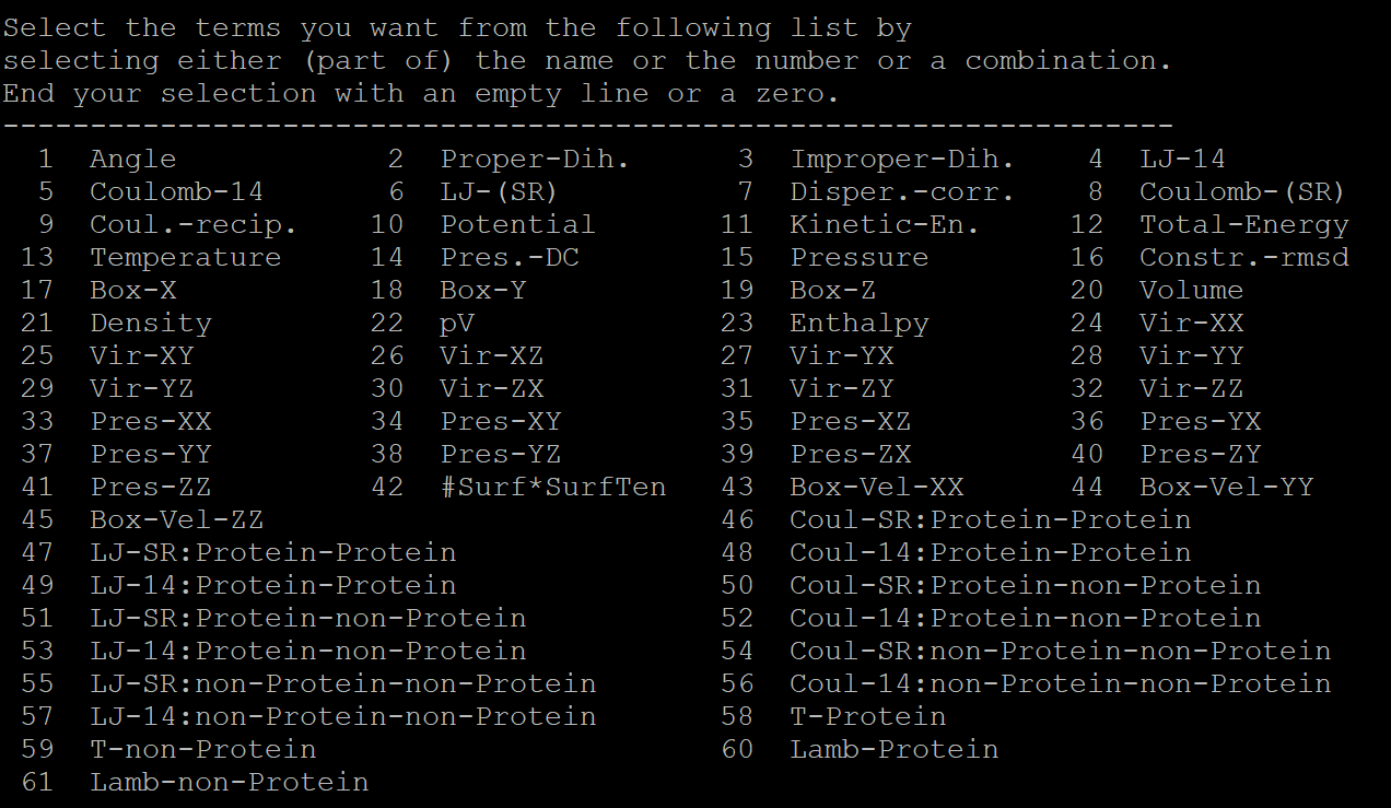
Here, we'd like to extract the energy and temperature data, so we type 10 11 12 13 and key in Enter twice to execute the operation.

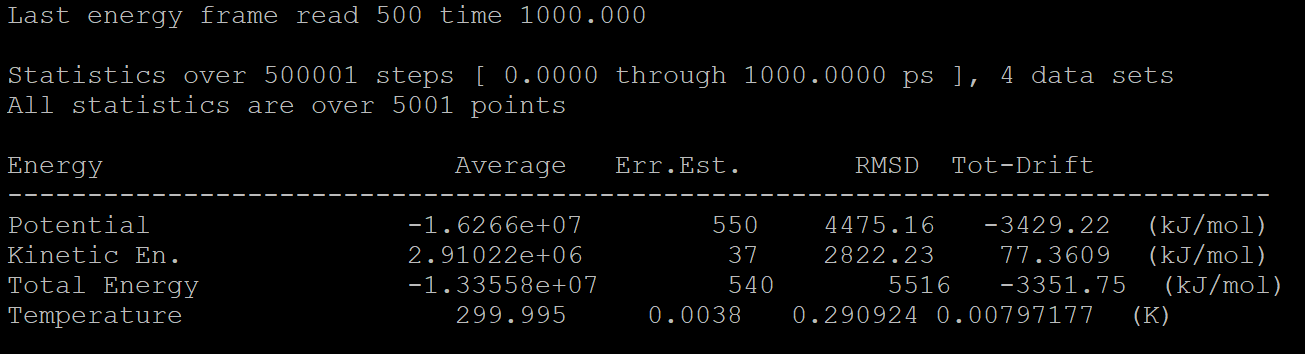
The result will show in cns1_enrg-npt.xvg, and we can draw the picture using Microsoft Office Excel.

2.4.3 Alignment to the initial structure

Firstly, we need to convert the cns1_npt-nopr.pro to pdb file.

gmx editconf -f cns1_npt-nopr.gro -o cns1_npt-nopr.pdb

Use align operation in Pymol to align the two structures

Aftering loading the structures into pymol software, we should remove the waters and ions of the MD result structure.

In pymol, on the right bar of cns1_npt-nopr, click action|remove waters to remove waters, and alert the selecting state of Residue on the bottom right to Molecule.

Click on the protein molecule and it appears an object called (sele), and click action|extract object and it created an object called obj01. Rename it to cns1_MD.

Load the initial structure file cns1_model1.pdb and we can align the two structures.

align cns1_MD, cns1_model1

After alignment, we can get the RMSD value in the console.

If we want to make a movie of the 360-degree-view about the alignment, we need to use pymol console.

PyMOL> mset 1 x360
This command creates a movie with 60 frames
PyMOL> util.mroll 1,360
This command rotates the protein molecule 360 deg in 360 frames
#the number of the frames can control the speed of the rotation, more frames means lower speed.
PyMOL> mplay
Type "mstop" to stop the animation
2. Saving frames in PNG format
PyMOL> mpng frame

It saves 360 frames png file in the python36 directory, use VideoMach to generate gif file.

2.4.4 Calculation of RMSD fluctuation

Use gmx rms to calculate the RMSD between the backbone after molecular dynamics simulation and the initial backbone.

gmx rms -s cns1_npt-nopr.tpr -f cns1_npt-nopr.xtc -o cns1-bkbone-rmsd.xvg

Choose option 4 (backbone) when it alerts.

Use gmx rmsdist to calculate the RMSD of the distance fluctuation betwwen the atoms.

gmx rmsdist -s cns1_npt-nopr.tpr -f cns1_npt-nopr.xtc -o cns1_distrmsd.xvg

Likewise, use Excel to draw the picture.