Protein-Ligand Simulation Using GROMACS

Protein-Ligand complex simulation GROMACS

Software: GROMACS

GROMACS Manual

Platform: Linux

Initial Protein: HisG_MD.pdb

Initial Ligand: ADN.pdb

1 Check GROMACS

GROMACS location:

/usr/local/gromacs/bin/

Set environment variable:

export PATH=$PATH:/usr/local/gromacs/bin/
#test if environment works
gmx -version

2 HisG-Adenosine complex MD Simulation

2.1 Prepare Molecular Topology file

As the long time consumed in this simulation, we only conduct the simulation for HisG. Since we have conducted Molecular Dynamics Simulation of the enzyme cns1, cns2, cns3 and its HisG domain, we'd like to use the result structure as the input protein file. For cns3-HisG domain we call it HisG_MD.pdb.

The first thing to do is to find and download the ligand structure, here, we search "Adenosine" in PDBeChem and dowload the ".pdb" file, we call it ADN.pdb.

According to the manual, the ligand is not a recognized entity in any of the force fields provided with GROMACS, so we can not use pdb2gmx to generate the topology of the ligand.

The force field we will be using in this tutorial is CHARMM36, obtained from the MacKerell lab website. While there, download the latest CHARMM36 force field tarball and the "cgenff_charmm2gmx.py" conversion script, which we will use later. Download the version of the conversion script that corresponds to your installed Python version (Python 2.x or 3.x).

Unarchive the force field tarball in your working directory:

tar -zxvf charmm36-mar2019.ff.tgz

There should now be a "charmm36-mar2019.ff" subdirectory in your working directory.

2.1.1 Generate the protein topology

Then, Write the topology for HisG with pdb2gmx:

gmx pdb2gmx -f HisG_MD.pdb -ignh -o HisG_MD_processed.gro

In this operation, we ignore the water using -ignh or we will get a fatal error due to the inconsistence of the name of the water. Choose the default water model when prompted (TIP3P). The structure will be processed by pdb2gmx, and you will be prompted to choose a force field:

Choose the first force filed which is just installed by us manually, CHARMM36 all-atom force field (March 2019).

2.1.1 Generate the ligand topology

Let's move to deal with the ligand.

Here, we use CGenFF, an official CHARMM General Force Field server to generate the topology of the ligand.

Since the strict requirement of this online server on the file format of the ligand. We need to:

• Add Hydrogen Atoms to the ligand
• Convert the pdb file to mol2 file
• Several corrections to the generated mol2 file

We use avogadro to add the hydrogen atoms and convert it to mol2 format.

Open Adenosine.pdb in Avogadro, and from the "Build" menu, choose "Add Hydrogens." Avogadro will build all of the H atoms onto the Adenosine ligand. Save a .mol2 file (File -> Save As... and choose Sybyl Mol2 from the drop-down menu) named "ADN.mol2."

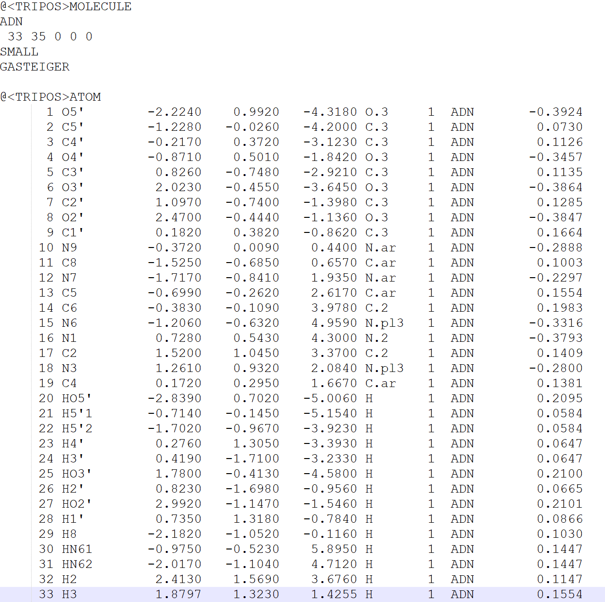
In order to correct the mol2 file, we need to look through it.

• Change the name of the molecule to Adenosine
• Change the sixth column to 1
• Change the seventh column to Adenosine
• Change the name of the atoms uniquely

Last, notice the strange bond order in the @BOND section. All programs seem to have their own method for generating this list, but not all are created equal. There will be issues in constructing a correct topology with matching coordinates if the bonds are not listed in ascending order. To fix this problem, download the sort_mol2_bonds.pl script and execute it:

Run the script to fix the bonds.

perl sort_mol2_bonds.pl ADN.mol2 ADN_fix.mol2

Use "ADN_fix.mol2" in the next step.

Now, we'd like to generate the topology of the ligand using CGenFF server.

The ADN_fix.mol2 file is now ready for use to produce a topology. Visit the CGenFF server, log into your account, and and click "Upload molecule" at the top of the page. Upload Adenosine_fix.mol2 and the CGenFF server will quickly return a topology in the form of a CHARMM "stream" file (extension .str). Save its contents from your web browser into a file called "ADN.str."

Check the penalty of the .str file carefully! If the penalty is high, please double check the original ligand file whether it is a valid structure.

Alter the resi name of the .str file of to ADN, or it will create error in the next step.

Then we use the python script to generate the topology:

python cgenff_charmm2gmx.py ADN ADN_fix.mol2 ADN.str charmm36-mar2019.ff

If we do not alter the name of the RESI (the figure below),

we will get the error:

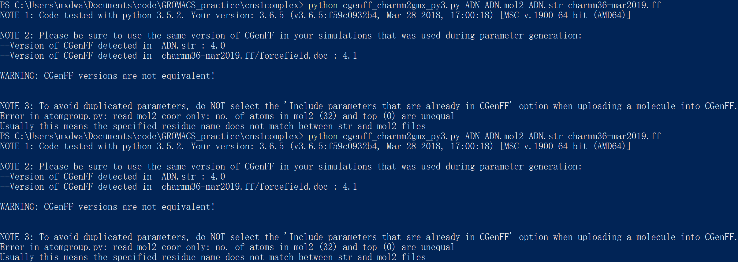
It means that the mol2 file and the str file is not consistent.

When we successfully run the transcript, we will get the result below:

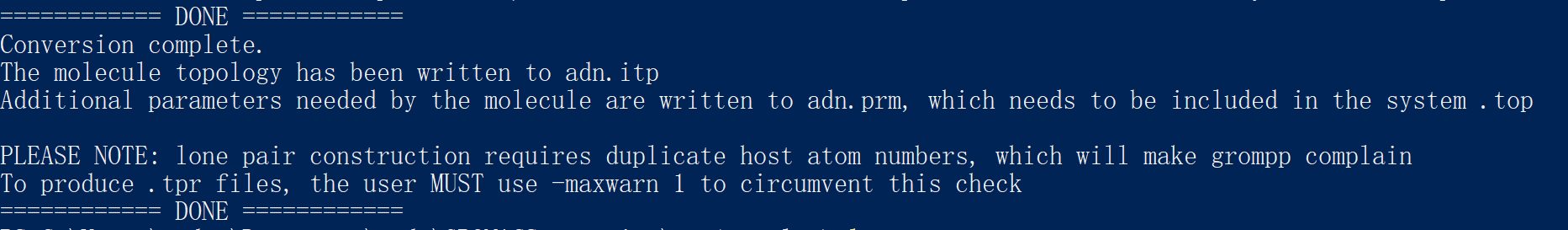
We get adn.itp, adn.prm, adn.top, adn_ini.pdb.

We convert the adn_ini.pdb to adn.gro using editconf:

gmx editconf -f adn_ini.pdb -o adn.gro

2.2 Build Complex Topology file

Copy HisG_MD_processed.gro to a new file to be manipulated, for instance, call it "complex.gro," as the addition of ADN to the protein will generate our protein-ligand complex. Next, simply copy the coordinate section of adn.gro and paste it into complex.gro, below the last line of the protein atoms, and before the box vectors, like so:

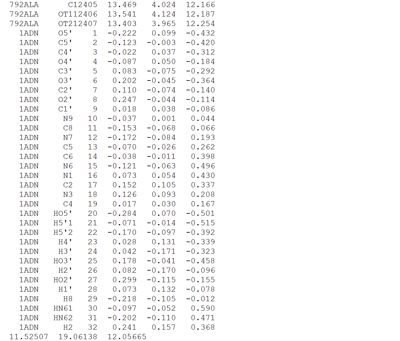
Since we add 32 atoms into the .gro file, increment the second line of complex.gro to reflect this change. There should be 12439 atoms in the coordinate file now.

Insert a line that says #include "adn.itp" into topol.top after the position restraint file is included. The inclusion of position restraints indicates the end of the "Protein" moleculetype section.

; Include Position restraint file
#ifdef POSRES
#include "posre.itp"
#endif
; Include water topology
#include "./charmm36-mar2019.ff/tip3p.itp"

becomes

; Include Position restraint file
#ifdef POSRES
#include "posre.itp"
#endif
; Include ligand topology
#include "adn.itp"
; Include water topology
#include "./charmm36-mar2019.ff/tip3p.itp"

The ligand introduces new dihedral parameters, which were written to "adn.prm" by the cgenff_charmm2gmx_py3.py script. At the TOP of topol.top, insert an #include statement to add these parameters:

; Include forcefield parameters
#include "./charmm36-mar2019.ff/forcefield.itp"
; Include ligand parameters
#include "adn.prm"
[ moleculetype ]
; Name            nrexcl
Protein_chain_A     3

The last adjustment to be made is in the [ molecules ] directive. To account for the fact that there is a new molecule in complex.gro, we have to add it here, like so:

[ molecules ]
; Compound        #mols
Protein_chain_A     1
ADN                 1

Remember to substitude the original topol.top with the updated one.

2.3 MD Simulation

At this point, the workflow is just like any other MD simulation. We will define the unit cell and fill it with water.

gmx editconf -f complex.gro -o newbox.gro -bt dodecahedron -d 1.0
gmx solvate -cp newbox.gro -cs spc216.gro -p topol.top -o solv.gro

Use em.mdp to build the ion.tpr and conduct energy minimization:

em.mdp:

; LINES STARTING WITH ';' ARE COMMENTS
title           = Minimization  ; Title of run
; Parameters describing what to do, when to stop and what to save
integrator      = steep     ; Algorithm (steep = steepest descent minimization)
emtol           = 1000.0    ; Stop minimization when the maximum force < 10.0 kJ/mol
emstep          = 0.01      ; Energy step size
nsteps          = 50000     ; Maximum number of (minimization) steps to perform
; Parameters describing how to find the neighbors of each atom and how to calculate the interactions
nstlist         = 1             ; Frequency to update the neighbor list and long range forces
cutoff-scheme   = Verlet
ns_type         = grid          ; Method to determine neighbor list (simple, grid)
rlist           = 1.2           ; Cut-off for making neighbor list (short range forces)
coulombtype     = PME           ; Treatment of long range electrostatic interactions
rcoulomb        = 1.2           ; long range electrostatic cut-off
vdwtype         = cutoff
vdw-modifier    = force-switch
rvdw-switch     = 1.0
rvdw            = 1.2           ; long range Van der Waals cut-off
pbc             = xyz           ; Periodic Boundary Conditions
DispCorr        = no

Type the code:

gmx grompp -f em.mdp -c solv.gro -p topol.top -o ion.tpr

We now pass our .tpr file to genion:

gmx genion -s ion.tpr -o solv_ions.gro -p topol.top -pname NA -nname CL -neutral

In order to run energy minimization by mdrun, we have to use the grompp operation again.

gmx grompp -f em.mdp -c solv_ions.gro -p topol.top -o HisGcomplex_em.tpr

Then, we run energy minimization:

gmx mdrun -v -deffnm HisGcomplex_em

Before conducting equilibration, we need to apply restraints to the ligand and do the treatment of temperature coupling groups.

gmx make_ndx -f adn.gro -o index_adn.ndx
> 0 & ! a H*
> q

Then, execute the genrestr module and select this newly created index group (which will be group 3 in the index_jz4.ndx file):

gmx genrestr -f adn.gro -n index_adn.ndx -o posre_adn.itp -fc 1000 1000 1000

Now, we need to include this information in our topology. We can do this in several ways, depending upon the conditions we wish to use. If we simply want to restrain the ligand whenever the protein is also restrained, add the following lines to your topology in the location indicated:

; Include Position restraint file
#ifdef POSRES
#include "posre.itp"
#endif
; Include ligand topology
#include "adn.itp"
; Ligand position restraints
#ifdef POSRES
#include "posre_adn.itp"
#endif
; Include water topology
#include "./charmm36-mar2019.ff/tip3p.itp"

gmx make_ndx -f HisGcomplex-em.gro -o index.ndx

Merge the "Protein" and "ADN" groups with the following, where ">" indicates the make_ndx prompt:

> 1 | 13
> q

Proceed with NVT equilibration using this .mdp file.

title                   = Protein-ligand complex NVT equilibration 
define                  = -DPOSRES  ; position restrain the protein and ligand
; Run parameters
integrator              = md        ; leap-frog integrator
nsteps                  = 50000     ; 2 * 50000 = 100 ps
dt                      = 0.002     ; 2 fs
; Output control
nstenergy               = 500   ; save energies every 1.0 ps
nstlog                  = 500   ; update log file every 1.0 ps
nstxout-compressed      = 500   ; save coordinates every 1.0 ps
; Bond parameters
continuation            = no        ; first dynamics run
constraint_algorithm    = lincs     ; holonomic constraints 
constraints             = h-bonds   ; bonds to H are constrained 
lincs_iter              = 1         ; accuracy of LINCS
lincs_order             = 4         ; also related to accuracy
; Neighbor searching and vdW
cutoff-scheme           = Verlet
ns_type                 = grid      ; search neighboring grid cells
nstlist                 = 20        ; largely irrelevant with Verlet
rlist                   = 1.2
vdwtype                 = cutoff
vdw-modifier            = force-switch
rvdw-switch             = 1.0
rvdw                    = 1.2       ; short-range van der Waals cutoff (in nm)
; Electrostatics
coulombtype             = PME       ; Particle Mesh Ewald for long-range electrostatics
rcoulomb                = 1.2       ; short-range electrostatic cutoff (in nm)
pme_order               = 4         ; cubic interpolation
fourierspacing          = 0.16      ; grid spacing for FFT
; Temperature coupling
tcoupl                  = V-rescale                     ; modified Berendsen thermostat
tc-grps                 = Protein_JZ4 Water_and_ions    ; two coupling groups - more accurate
tau_t                   = 0.1   0.1                     ; time constant, in ps
ref_t                   = 300   300                     ; reference temperature, one for each group, in K
; Pressure coupling
pcoupl                  = no        ; no pressure coupling in NVT
; Periodic boundary conditions
pbc                     = xyz       ; 3-D PBC
; Dispersion correction is not used for proteins with the C36 additive FF
DispCorr                = no 
; Velocity generation
gen_vel                 = yes       ; assign velocities from Maxwell distribution
gen_temp                = 300       ; temperature for Maxwell distribution
gen_seed                = -1        ; generate a random seed

Remember to change the nvt.mdp file according to the protein name in the line tc-grps = Protein_JZ4 Water_and_ions to tc-grps = Protein_ADN Water_and_ions

gmx grompp -f nvt.mdp -c HisGcomplex-em.gro -r HisGcomplex-em.gro -p topol.top -n index.ndx -o HisGcomplex-nvt.tpr
nohup gmx mdrun -deffnm HisGcomplex-nvt &
#tail -n 25 HisGcomplex-nvt.log

NPT equilibrium

title                   = Protein-ligand complex NPT equilibration 
define                  = -DPOSRES  ; position restrain the protein and ligand
; Run parameters
integrator              = md        ; leap-frog integrator
nsteps                  = 50000     ; 2 * 50000 = 100 ps
dt                      = 0.002     ; 2 fs
; Output control
nstenergy               = 500       ; save energies every 1.0 ps
nstlog                  = 500       ; update log file every 1.0 ps
nstxout-compressed      = 500       ; save coordinates every 1.0 ps
; Bond parameters
continuation            = yes       ; continuing from NVT 
constraint_algorithm    = lincs     ; holonomic constraints 
constraints             = h-bonds   ; bonds to H are constrained 
lincs_iter              = 1         ; accuracy of LINCS
lincs_order             = 4         ; also related to accuracy
; Neighbor searching and vdW
cutoff-scheme           = Verlet
ns_type                 = grid      ; search neighboring grid cells
nstlist                 = 20        ; largely irrelevant with Verlet
rlist                   = 1.2
vdwtype                 = cutoff
vdw-modifier            = force-switch
rvdw-switch             = 1.0
rvdw                    = 1.2       ; short-range van der Waals cutoff (in nm)
; Electrostatics
coulombtype             = PME       ; Particle Mesh Ewald for long-range electrostatics
rcoulomb                = 1.2
pme_order               = 4         ; cubic interpolation
fourierspacing          = 0.16      ; grid spacing for FFT
; Temperature coupling
tcoupl                  = V-rescale                     ; modified Berendsen thermostat
tc-grps                 = Protein_JZ4 Water_and_ions    ; two coupling groups - more accurate
tau_t                   = 0.1   0.1                     ; time constant, in ps
ref_t                   = 300   300                     ; reference temperature, one for each group, in K
; Pressure coupling
pcoupl                  = Berendsen                     ; pressure coupling is on for NPT
pcoupltype              = isotropic                     ; uniform scaling of box vectors
tau_p                   = 2.0                           ; time constant, in ps
ref_p                   = 1.0                           ; reference pressure, in bar
compressibility         = 4.5e-5                        ; isothermal compressibility of water, bar^-1
refcoord_scaling        = com
; Periodic boundary conditions
pbc                     = xyz       ; 3-D PBC
; Dispersion correction is not used for proteins with the C36 additive FF
DispCorr                = no 
; Velocity generation
gen_vel                 = no        ; velocity generation off after NVT 

Likewise, remember to change the nvt.mdp file according to the protein name in the line tc-grps = Protein_JZ4 Water_and_ions

gmx grompp -f npt.mdp -c HisGcomplex-nvt.gro -t HisGcomplex-nvt.cpt -r HisGcomplex-nvt.gro -p topol.top -n index.ndx -o HisGcomplex-npt.tpr
nohup gmx mdrun -deffnm HisGcomplex-npt &
#tail -n 25 HisGcomplex-npt.log

md.mdp

title                   = Protein-ligand complex MD simulation 
; Run parameters
integrator              = md        ; leap-frog integrator
nsteps                  = 5000000   ; 2 * 5000000 = 10000 ps (10 ns)
dt                      = 0.002     ; 2 fs
; Output control
nstenergy               = 10000      ; save energies every 20.0 ps
nstlog                  = 10000      ; update log file every 20.0 ps
nstxout-compressed      = 10000      ; save coordinates every 20.0 ps
; Bond parameters
continuation            = yes       ; continuing from NPT 
constraint_algorithm    = lincs     ; holonomic constraints 
constraints             = h-bonds   ; bonds to H are constrained
lincs_iter              = 1         ; accuracy of LINCS
lincs_order             = 4         ; also related to accuracy
; Neighbor searching and vdW
cutoff-scheme           = Verlet
ns_type                 = grid      ; search neighboring grid cells
nstlist                 = 20        ; largely irrelevant with Verlet
rlist                   = 1.2
vdwtype                 = cutoff
vdw-modifier            = force-switch
rvdw-switch             = 1.0
rvdw                    = 1.2       ; short-range van der Waals cutoff (in nm)
; Electrostatics
coulombtype             = PME       ; Particle Mesh Ewald for long-range electrostatics
rcoulomb                = 1.2
pme_order               = 4         ; cubic interpolation
fourierspacing          = 0.16      ; grid spacing for FFT
; Temperature coupling
tcoupl                  = V-rescale                     ; modified Berendsen thermostat
tc-grps                 = Protein_JZ4 Water_and_ions    ; two coupling groups - more accurate
tau_t                   = 0.1   0.1                     ; time constant, in ps
ref_t                   = 300   300                     ; reference temperature, one for each group, in K
; Pressure coupling 
pcoupl                  = Parrinello-Rahman             ; pressure coupling is on for NPT
pcoupltype              = isotropic                     ; uniform scaling of box vectors
tau_p                   = 2.0                           ; time constant, in ps
ref_p                   = 1.0                           ; reference pressure, in bar
compressibility         = 4.5e-5                        ; isothermal compressibility of water, bar^-1
; Periodic boundary conditions
pbc                     = xyz       ; 3-D PBC
; Dispersion correction is not used for proteins with the C36 additive FF
DispCorr                = no 
; Velocity generation
gen_vel                 = no        ; continuing from NPT equilibration 

Likewise, remember to change the nvt.mdp file according to the protein name in the line tc-grps = Protein_JZ4 Water_and_ions

gmx grompp -f md.mdp -c HisGcomplex-npt.gro -t HisGcomplex-npt.cpt -p topol.top -n index.ndx -o HisGcomplex-md_10ns.tpr
nohup gmx mdrun -deffnm HisGcomplex-md_10ns &
#tail -n 25 HisGcomplex-md_10ns.log

3 Result Analysis

3.1 Generate trace file

To recenter the protein and rewrap the molecules within the unit cell to recover the desired rhombic dodecahedral shape, invoke trjconv:

gmx trjconv -s HisGcomplex-md_10ns.tpr -f HisGcomplex-md_10ns.xtc -o HisGcomplex-md_10ns_center.xtc -center -pbc mol -ur compact

Choose "Protein" for centering and "System" for output. Note that centering complexes (protein-ligand, protein-protein) may be difficult for longer simulations involving many jumps across periodic boundaries. In those instances (particularly in protein-protein complexes), it may be necessary to create a custom index group to use for centering, corresponding to the active site of one protein or the interfacial residues of one monomer in a complex.

To extract the first frame (t = 0 ns) of the trajectory, use trjconv -dump with the recentered trajectory:

gmx trjconv -s HisGcomplex-md_10ns.tpr -f HisGcomplex-md_10ns_center.xtc -o HisGcomplex_start.pdb -dump 0

For even smoother visualization, it may be beneficial to perform rotational and translational fitting. Execute trjconv as follows:

gmx trjconv -s HisGcomplex-md_10ns.tpr -f HisGcomplex-md_10ns_center.xtc -o HisGcomplex-md_10ns_fit.xtc -fit rot+trans

Choose "Backbone" to perform least-squares fitting to the protein backbone, and "System" for output. Note that simultaneous PBC rewrapping and fitting of the coordinates is mathematically incompatible. Should you wish to perform fitting (which is useful for visualization, but not necessary for most analysis routines), carry out these coordinate manipulations separately, as indicated here.

3.2 Visualization

Transfer the xtc trace file into pdb file for visualization.

gmx trjconv -s HisGcomplex-md_10ns.gro -f HisGcomplex-md_10ns_fit.xtc -n index.ndx -o HisGcomplex_ADN-md_10ns_movie_fit.pdb

Using methods described in Molecular Dynamics Using GROMACS, users can generate trace video.

Enter 22 Protein-ADN to select both the structure of protein and ligand.

Change the gro structure to pdb structure.

gmx editconf -f HisGcomplex-md_10ns.gro -o HisGcomplex-md_10ns.pdb

Additional 1 nanosecond simulation, changing simulation time to 1ns in md1.mdp. And run:

gmx grompp -f md1.mdp -c HisGcomplex-md_10ns.gro -t HisGcomplex-md_10ns.cpt -p topol.top -n index.ndx -o HisGcomplex-md_Addi_1ns.tpr
nohup gmx mdrun -deffnm HisGcomplex-md_Addi_1ns &
#tail -n 25 HisGcomplex-md_Addi_1ns.log

Using visualization methods above to see the simulation process.