@TaoSama
2026-03-22T14:05:34.000000Z
字数 14697
阅读 1995
Coursera Machine Learning
Machine-Learning
click the top right button to show the content
0. Symbols
training examples, features
feature of example
1. Linear Regression
Hypothesis Function
Cost Function
Gradient Descent Algorithm
Simultaneous Update
2. Multivaritate Linear Regression
Hypothesis Function
Gradient Descent for Multiple Variables
Feature Scaling and Mean Normalization
- make fit in or
3 times is also ok, ... -
Where is the average of all the values for feature and is the range of values , or is the standard deviation.
Learning Rate
- If is too small: slow convergence.
- If is too large: may not decrease on every iteration and thus may not converge.
- To choose , try
Features and Polynomial Regression
- combine multiple features into one
- change feature to polynomial as a feature
- don't forget feature scaling
Normal Equation
, is matrix, is -dimensional vector
is to make a square matrix
- There is no need to do feature scaling with the normal equation.
- The following is a comparison of gradient descent and the normal equation:
Gradient Descent Normal Equation Need to choose alpha No need to choose alpha Needs many iterations No need to iterate , need to calculate inverse of Works well when n is large Slow if n is very large when is non-invertible:
- Redundant features, where two features are very closely related (i.e. they are linearly dependent)
- Too many features (e.g. ). In this case, delete some features or use "regularization" (to be explained in a later lesson).
3. Logistic Regression
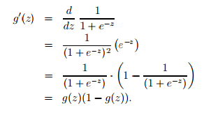
Hypothesis Function
"Sigmoid Function", also called the "Logistic Function":
Decision Boundary
-
- if is taken as input:
Cost Function
-
-
- Based on maximum liklihood estimation, simplify it:
A vectorized implementation is:
Gradient Descent
A vectorized implementation is:
Deduction:
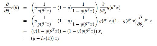
PS: it will be equal with a minus sign
Advanced Optimization
use matlab/Octave built-in libraries, such as fminunc()
function [jVal, gradient] = costFunction(theta, X, y)jVal = [...code to compute J(theta)...];gradient = [...code to compute derivative of J(theta)...];endoptions = optimset('GradObj', 'on', 'MaxIter', 100);initialTheta = zeros(2,1);[optTheta, functionVal, exitFlag] = ...fminunc(@(theta)(costFunction(theta, X, y)), initial_theta, options);
Multiclass Classification: One-vs-all
Train a logistic regression classifier for each class to predict the probability .
To make a prediction on a new , pick the class that maximizes
Overfitting
An instance of overfitting: a hypothesis having high variance and being unlikely to generalize well to new examples.
- Reduce the number of features:
- Manually select which features to keep.
- Use a model selection algorithm (studied later in the course).
- Regularization
- Keep all the features, but reduce the magnitude of parameters .
- Regularization works well when we have a lot of slightly useful features.
Regularization
Linear Regression
- Cost Function
The , or lambda, is the regularization parameter - Gradient Descent
with some manipulation:
- Normal Equation
PS: I don't know how to calculate it yet! A pity!
Logistic Regression
- Cost Function
- Gradient Descent
same as linear regression in form but different
4. Neural Networks
Model Representation
In neural networks, we use the same logistic function as in classification, , yet we sometimes call it a sigmoid (logistic) activation function. In this situation, our "theta" parameters are sometimes called "weights".
Visually, a simplistic representation looks like:
If network has units in layer and units in layer , then will be of dimension .
Setting , we can get the equation:
Cost Function
- = total number of layers in the network
- = number of units (not counting bias unit) in layer
- = number of output units/classes
Backpropagation Algorithm

Given training set
- Set for all
For training example :
- Set
- Perform forward propagation to compute for
- Using , compute
- Compute using
- or with vectorization,
Hence we update our new Δ matrix.
- Thus we get
Backpropagation in Practice
- Unrolling Parameters
% unrollthetaVector = [ Theta1(:); Theta2(:); Theta3(:); ]deltaVector = [ D1(:); D2(:); D3(:) ]% backTheta1 = reshape(thetaVector(1:110),10,11)Theta2 = reshape(thetaVector(111:220),10,11)Theta3 = reshape(thetaVector(221:231),1,11)
- Gradient Checking
make sure of only checking once
The approximate value of gradient:
a good way to choose epsilon is:
epsilon = 1e-4;for i = 1:n,thetaPlus = theta;thetaPlus(i) += epsilon;thetaMinus = theta;thetaMinus(i) -= epsilon;gradApprox(i) = (J(thetaPlus) - J(thetaMinus))/(2*epsilon)end;
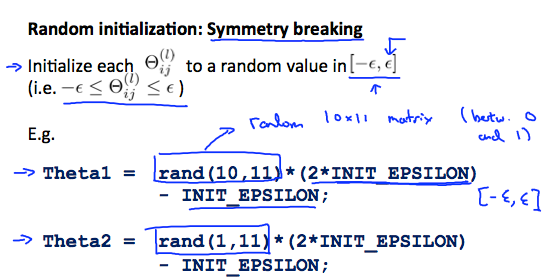
- Random Initialization
5. Evaluating a Learning Algorithm
Evaluating a Hypothesis
Once we have done some trouble shooting for errors in our predictions by:
- Getting more training examples
- Trying smaller sets of features
- Trying additional features
- Trying polynomial features
- Increasing or decreasing
The test set error
- For linear regression:
- For classification ~ Misclassification error (aka 0/1 misclassification error):
The average test error for the test set is:
Model Selection and Train/Validation/Test Sets
One way to break down our dataset into the three sets is:
- Training set: 60%
- Cross validation set: 20%
- Test set: 20%
We can now calculate three separate error values for the three different sets using the following method:
- Optimize the parameters in using the training set for each polynomial degree.
- Find the polynomial degree d with the least error using the cross validation set.
- Estimate the generalization error using the test set with , ( from polynomial with lower error);
This way, the degree of the polynomial d has not been trained using the test set.
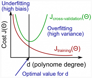
Bias vs. Variance
Diagnosing Bias vs. Variance
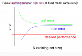
- High bias (underfitting): both and will be high. Also, .
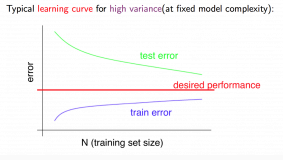
- High variance (overfitting): will be low and will be much greater than .
Regularization and Bias/Variance
- Create a list of s (i.e. ,0.01,0.02,0.04,0.08,0.16,0.32,0.64,1.28,2.56,5.12,10.24);
Create a set of models with different degrees or any other variants. - Iterate through the s and for each go through all the models to learn some .
- Compute the cross validation error using the learned (computed with λ) on the without regularization or .
- Select the best combo and that produces the lowest error on the cross validation set.
- Using the best combo, apply it on to see if it has a good generalization of the problem.
Learning Curves
Deciding What to Do Next Revisited
- Getting more training examples: Fixes high variance
- Trying smaller sets of features: Fixes high variance
- Adding features: Fixes high bias
- Adding polynomial features: Fixes high bias
- Decreasing λ: Fixes high bias
- Increasing λ: Fixes high variance.
System Design
Prioritizing What to Work On
- Collect lots of data (for example "honeypot" project but doesn't always work)
- Develop sophisticated features (for example: using email header data in spam emails)
- Develop algorithms to process your input in different ways (recognizing misspellings in spam).
It is difficult to tell which of the options will be most helpful.
Error Analysis
- Start with a simple algorithm, implement it quickly, and test it early on your cross validation data.
- Plot learning curves to decide if more data, more features, etc. are likely to help.
- Manually examine the errors on examples in the cross validation set and try to spot a trend where most of the errors were made.
Handling Skewed Class
- Error Metrics
| \ | Actual Class: 1 | Actual Class: 0 |
|---|---|---|
| Predicted Class: 1 | True Positive | False Positive |
| Predicted Class: 0 | False Negative | True Negative |
- Trade Off of Precision and Recall
Score
Using Large Data Sets
Rationale:
Useful test: Given the input , can a human expert confidently predict ?
- Use a learning algorithm with many parameters
- Use a very large training set (unlikely to overfit)
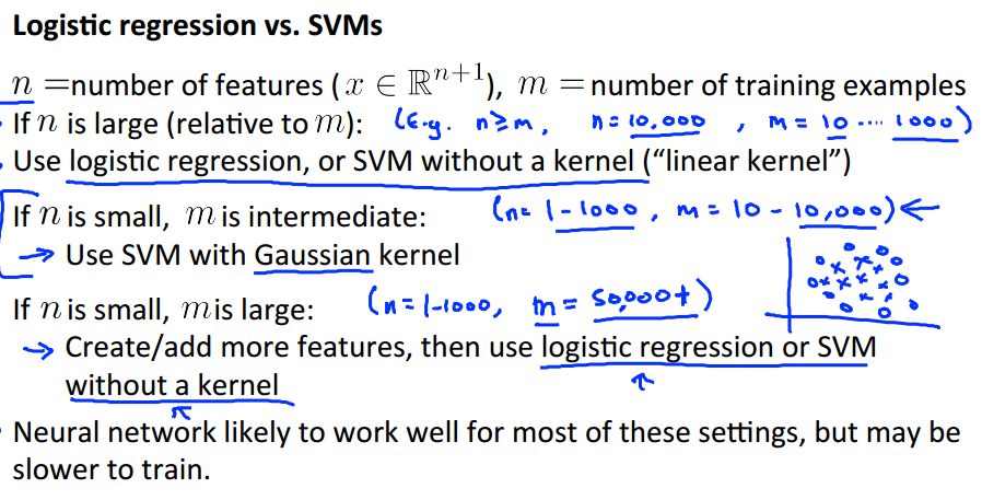
6. Support Vector Machines
Large Margin Classification
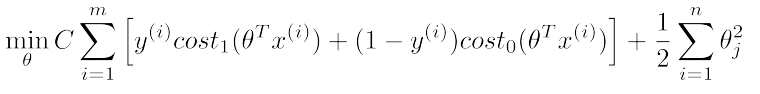
SVM Hypothesis
Large Margin Intuition
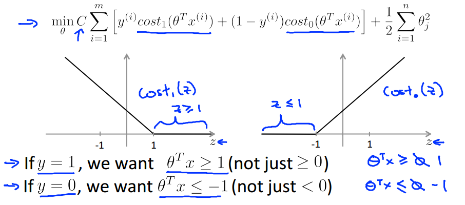
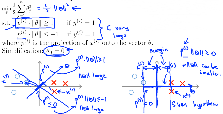
SVM Decision Boundary
can be small, then is going to be large, that is large margin.
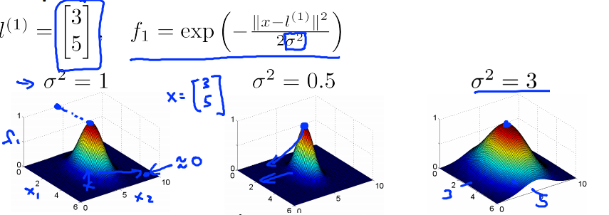
Kernels
Kernels ans Similarity
we define the similarity between and landmark as:
- ,
- ,
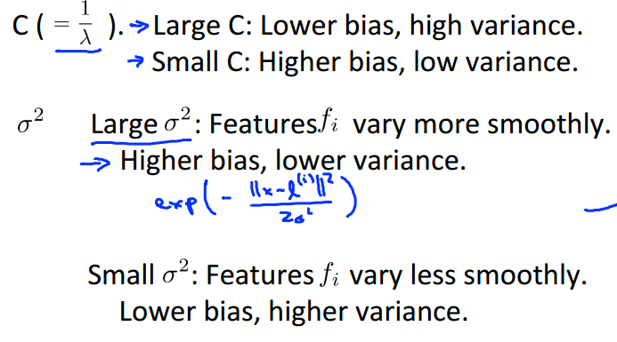
SVM Parameters
SVMs in Practice
7. Clustering
K-Means Algorithm
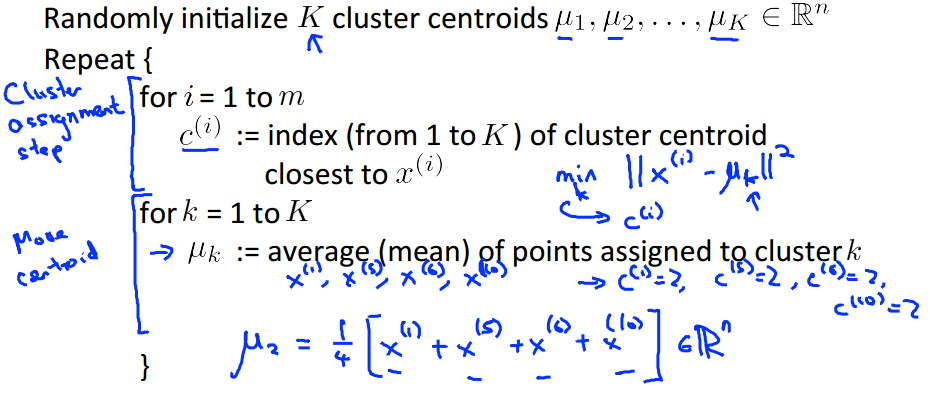
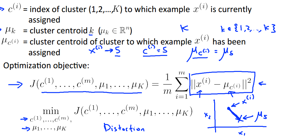
K-Means Optimization Objective
Random Initialization
- Should have
- Randomly pick training examples.
- Set equal to these examples.
Random initialization some times to pick the lowest cost one.
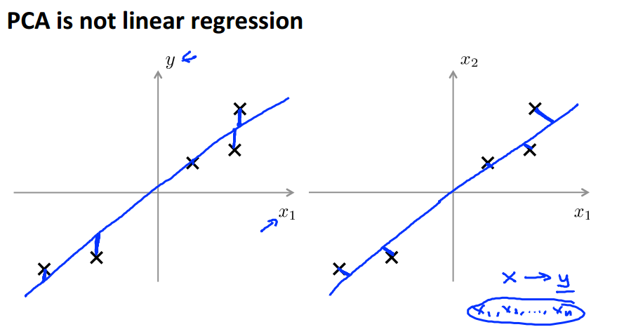
Principle Component Analysis
PCA is unsupervised learning, while LR is supervised learning
PCA Algorithm
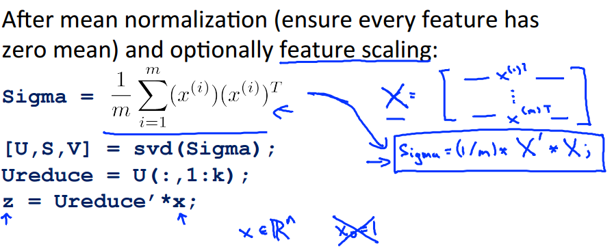
- Reconstruction from Compressed Representation
Dimensionality Reduc1on
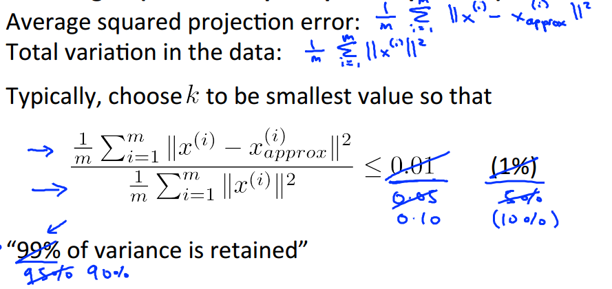
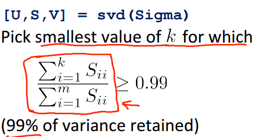
- Choosing the Number of Principal Components
Application of PCA
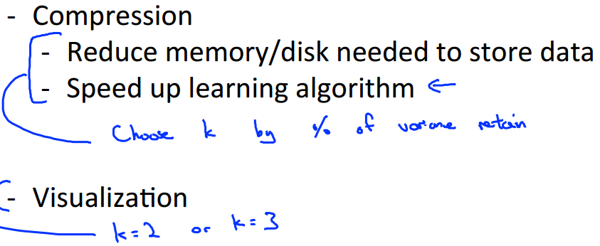
Bad use of PCA: To prevent overfitting
This might work OK, but isn’t a good way to address overfitting.
Use regularization instead. PCA lost the information of
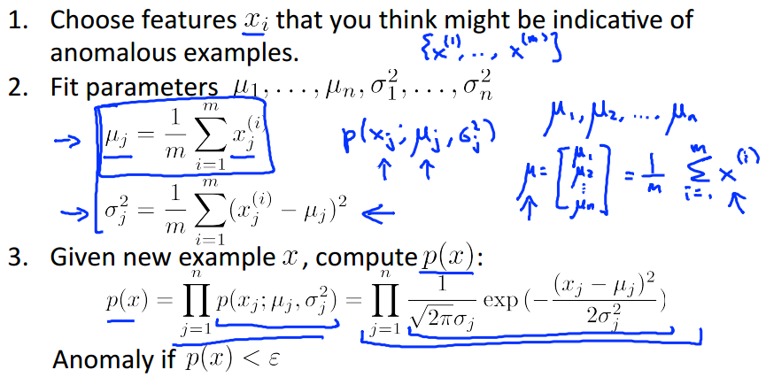
8. Anomaly Detection
Anomaly Detection Algorithm
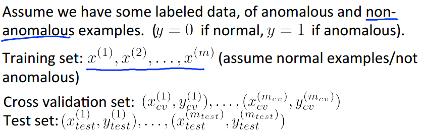
Evaluation
can use the same metrics or method as the algorithm before
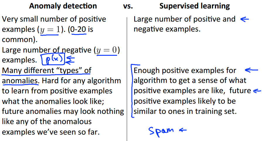
Anomaly Detection vs. Supervised Learning
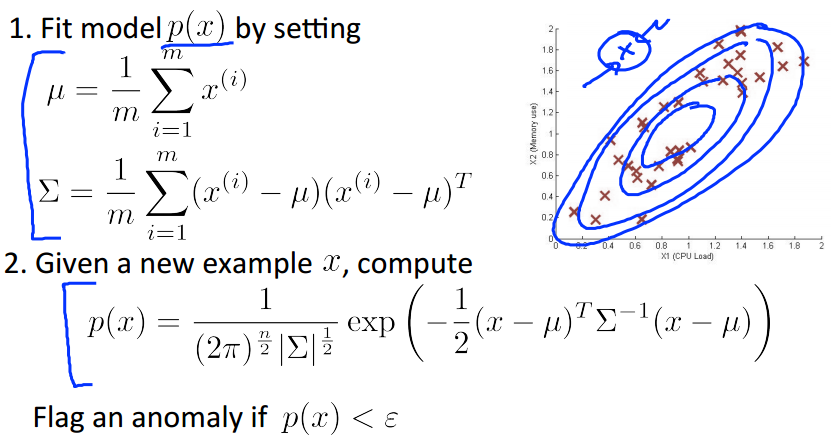
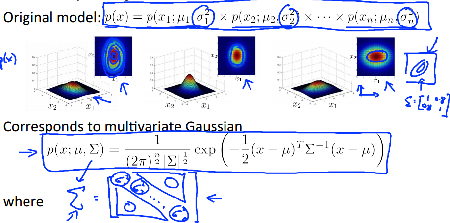
Anomaly Detectioon with the Multivariate Gaussian
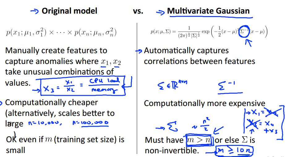
Relation to Original Model
- Diagnal Covariance Matrix
- Axis-aligned Figure
Original Model vs. Multivariate Gaussian
Recommender Systems
Content-based Recommender Systems
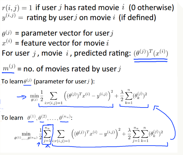
Collaborative Filtering
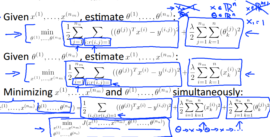
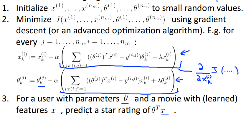
Collaborative Filtering Algorithm
mean normalization, to make the undefined value be predicted meaningfully
9. Large Scale Machine Learning
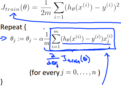
Gradient Descent with Large Datasets
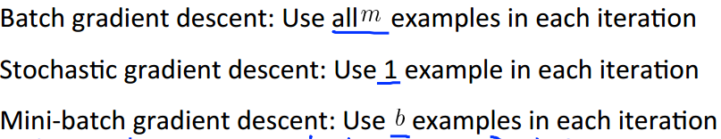
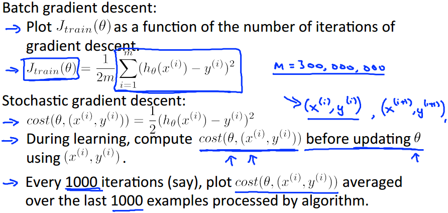
Batch Gradient Descent
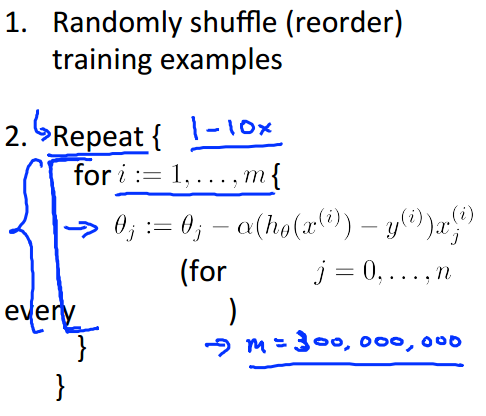
Stochastic Gradient Descent
- Learning Rate
It is not recommended, cuz adjusting 2 constants is a headache!

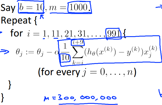
Mini-Batch Gradient Descent
Comparison
Checking forConvergence
Online Learning
- Its datasets is a continuous stream
- So get a example, update(gradient descent) once
- Can adopt to changing users' preference
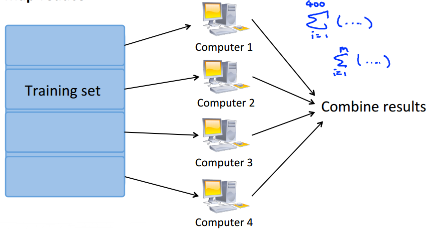
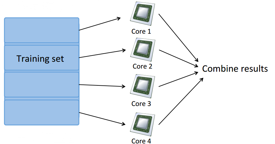
Map Reduce and Data Parallelism
- Map-reduce and summation over the training set
multiple machines:
multiple cores:
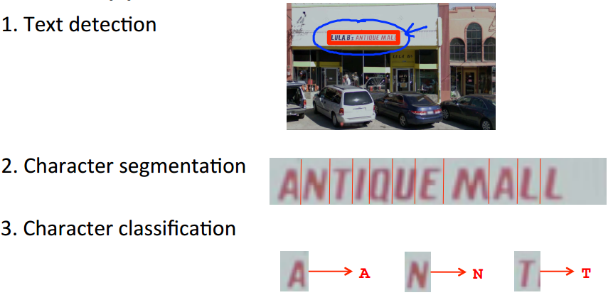
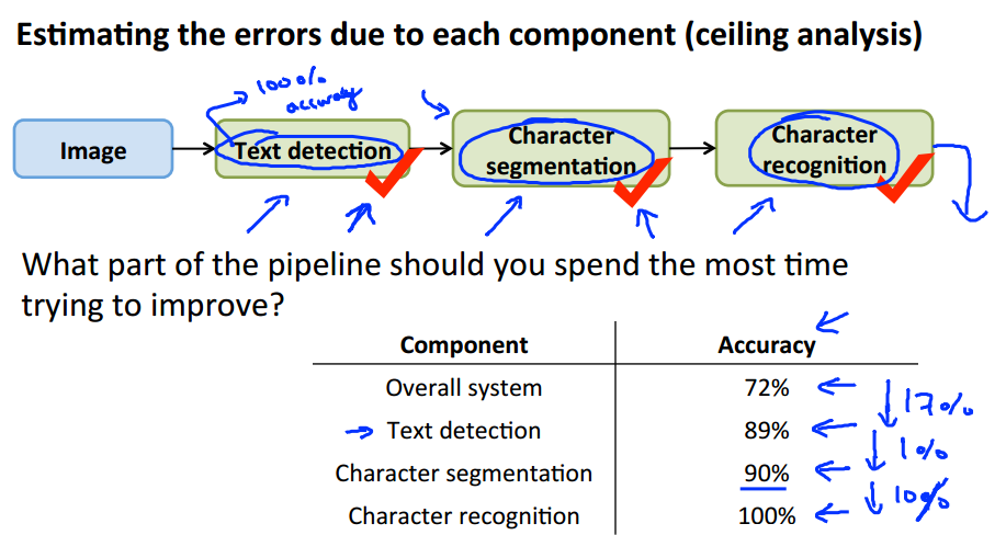
10. Application Example: Photo OCR
Photo OCR Pipeline
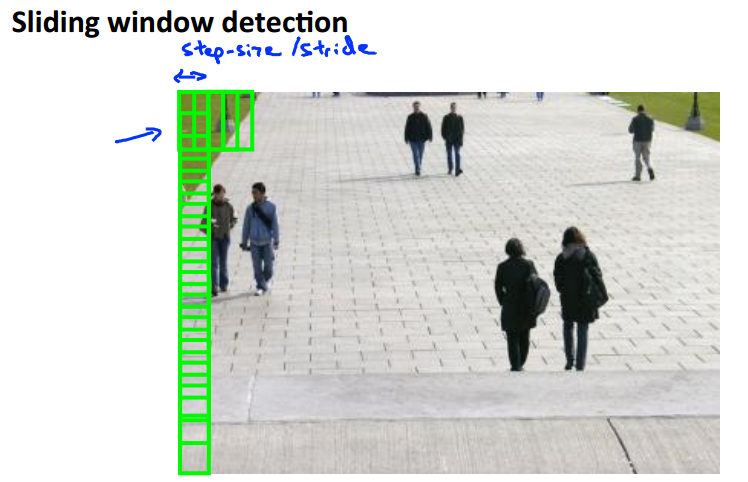
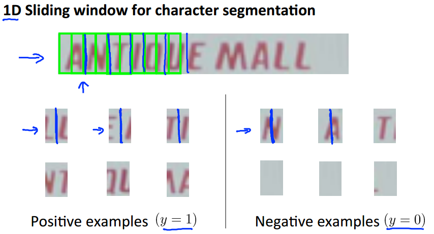
Sliding Windows
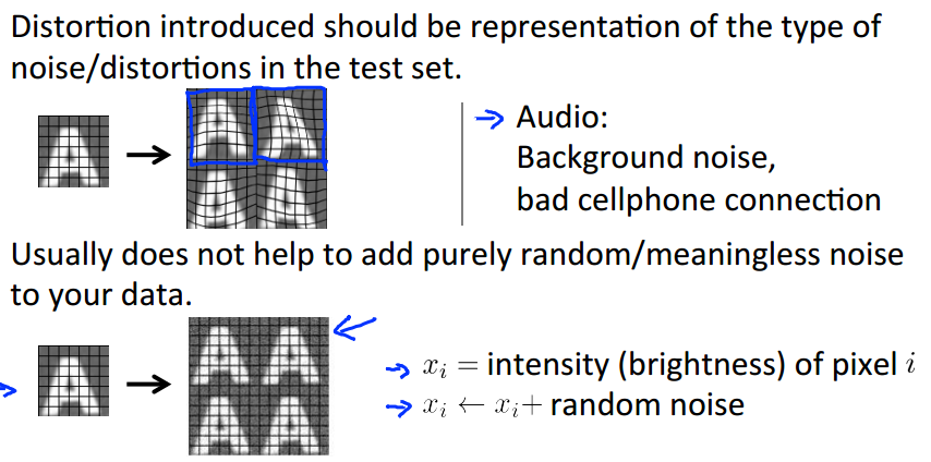
Getting Lots of Data and Artifical Data
Synthesizing data by introducing distortions
Discussion on Getting More Data
- Make sure you have a low bias classifier before expending the
effort. - How much work would it be to get 10x as much data as we currently have?
Ceiling Analysis: What Part of the Pipeline to Work on Next
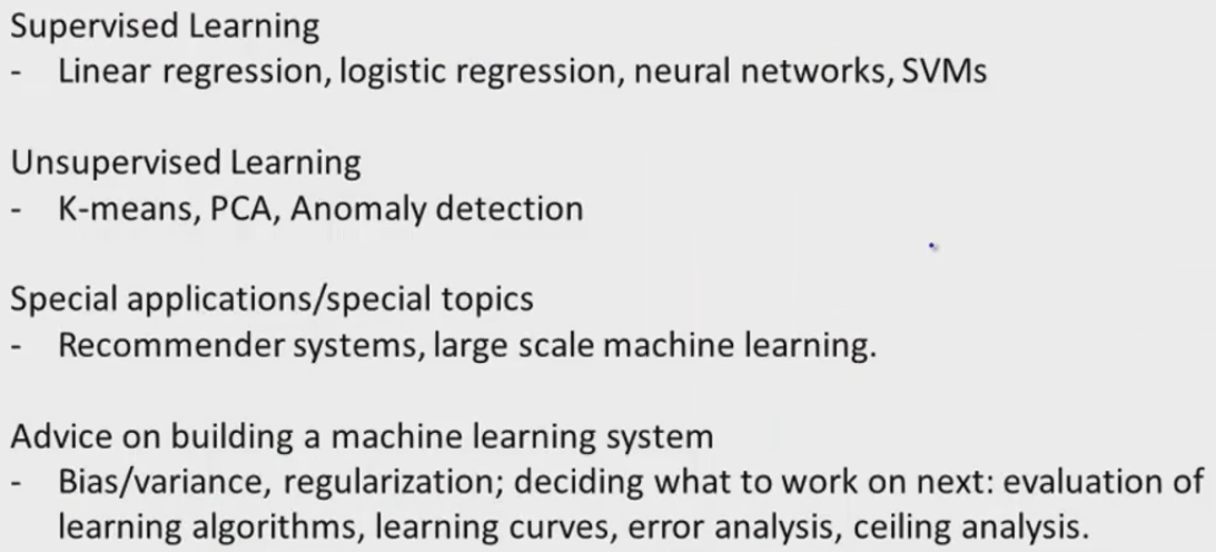
11. Summary: Main Topics