Random Systems

python homework

---

Abstuct

In this final exercise, I choose to discuss Chepter 7, the random system. First, I discuss two simple models, random walk in one dimension with fixed step length and random lengths. Then consider self-avoiding walks and cream-in-your-coffee model and draw the figure of entropy versus time.

Introduction and Background

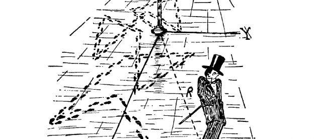
A random walk is a mathematical object which describes a path that consists of a succession of random steps. For example, the path traced by a molecule as it travels in a liquid or a gas, the search path of a foraging animal, superstring behavior, the price of a fluctuating stock and the financial status of a gambler can all be approximated by random walk models, even though they may not be truly random in reality. As illustrated by those examples, random walks have applications to many scientific fields including ecology, psychology, computer science, physics, chemistry, and biology, and also to economics. Random walks explain the observed behaviors of many processes in these fields, and thus serve as a fundamental model for the recorded stochastic activity. As a more mathematical application, the value of pi can be approximated by the usage of random walk in agent-based modelling environment.1 The term random walk was first introduced by Karl Pearson in 1905.

Content

1. Random walks
Here I draw the trajectories of a random walker in 2 demention. Code

First, we cosnider a situaion of one dimensional random walk.

The walker begins at the origin, $x = 0$, and the next step is chosen at random to be either right or left, each with probability 1/2. The step length we take is 1(right) or -1(left). I draw the figure 1.
Figure 1 Code

Left: x versus step number ,that is, for two random walks in one dimension. Right: $<x^2>$ as a function of step number (which is proportional to time) for a collection of one-dimensional randomn walks. The step length was unity and the results for 500 walkers were averaged. The points are the calculated values and the straight red line is a least-squares fit to the form:

$$<x^2>=2Dt \tag{1}$$
Then we generalize the model to make it more realistic. Allow the steps to be of random lengths. I have Figure 2.
Figure 2 Code

Here the steps were of random lengths in range -1 to 1.
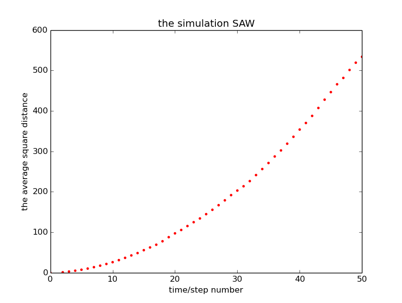
2. Self-Avoiding Walks
To investigate the shape of the macromolecule it is line-shaped,but can not intersect which means in one location can only be occupied once. We only investigate the two dimension SAW. In this case,we devise the SAW model, that is the path of the random walk particle will not pass the location which it has passed before. To accomplish this target, we must scan the location of the previous steps to see whether it has occupied the four location adjacent to the present particle location. if some has been taken up,the particle now can not pass them.
There are two methods to achieve this goal: one is simulation the other is enumeration. Simulation is first produce many random walk path step by step and if it has been self-intersect, then abandon them, so the rest can be all SAW path. Enumeration is the method to list the possible SAW path step by step.
Simulation approach,we finally get more than 200 SAW path in step 50, and get their average square distance. Due to the relation:$<r^2> =At^{2v}$ we exam the exact value of the v.
Figure 3

Enumeration approach, we use the previous scanning principle step by step to get the all possible path of SAW. Due the large number of calculation, we only do ten step. And our result perfectly agree with the list on the textbook. Since the average square distance has the relation:
$$\frac{<r^2_{n+1}>}{<r^2_n>}\sim 1+\frac{2v}{n}\tag{2}$$
Figure 4

this is the results by averaging all possible SAW path step by step
Figure 5

We can say the number of possible SAW path increase rapidly versus time and that is the reason for I only do 11 steps. Due to the relation (2).
Figure 6

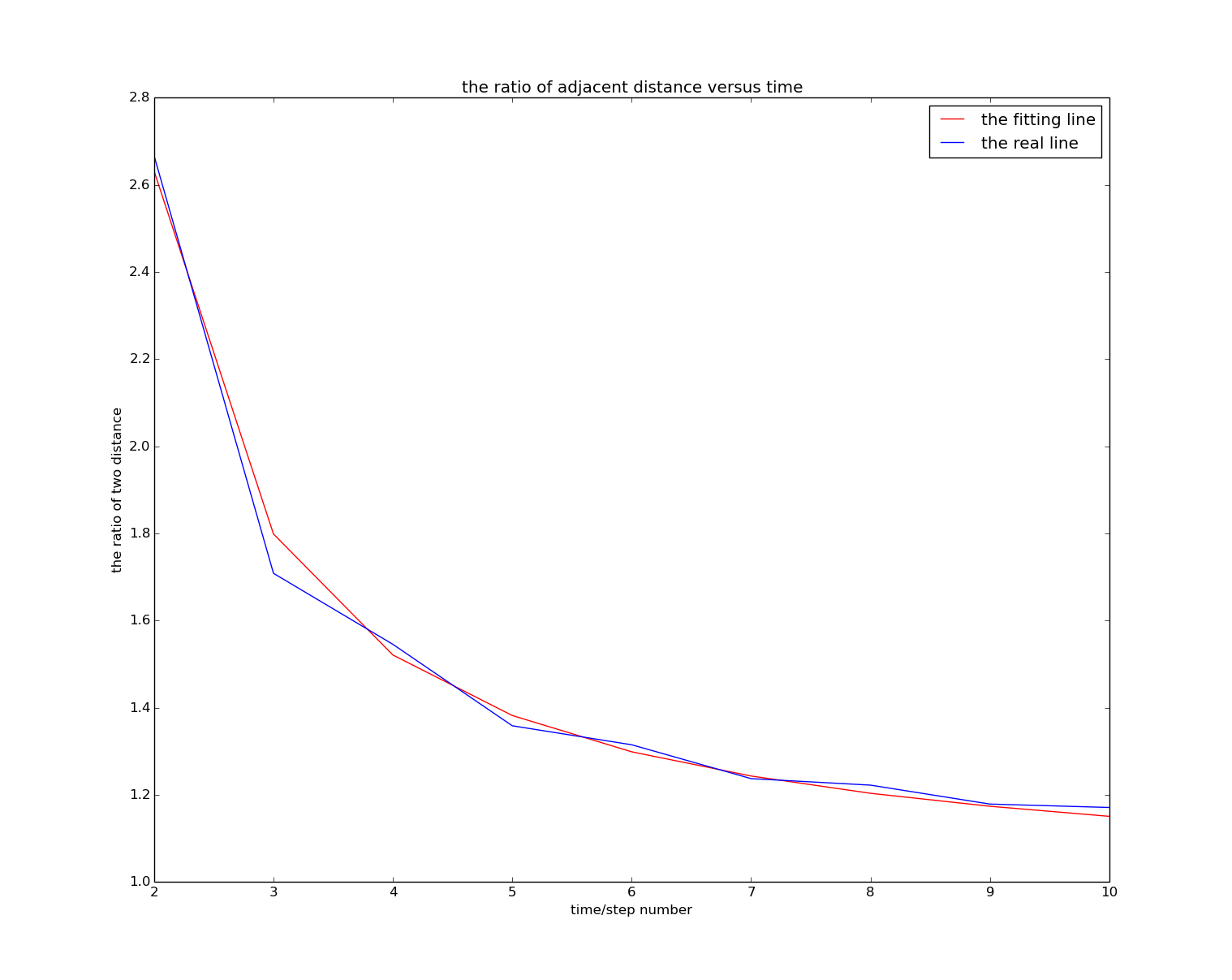
The equation of the fitting line is y=1.666/n+0.9654, So the v value is 0.833
Code

3. Random Walks and Diffusion
We know that random walks are equivalent to diffusion. We will adopt the cream-in-your-coffee analogy in which we have a large number of particles (cream) moving in solution (coffee). Calculate the density of particles $\rho$ varies as a function of time we have the diffusion equation:

$$\rho (i,n+1)=\rho (i,n)+\frac{D\Delta t}{(\Delta t)^2}[\rho (i+1,n)+\rho (i-1,n)-2\rho (i,n)]\tag{3}$$
As shown in figure 7.
Figure 7 Code

Now we consider 2 dimension. As shown in figure 8
Figure 8 Code



We can see that the particles "spread" as t inceases.

4. Diffusion, Entropy, and The Arrow of Time
Consider the cream-in-your-coffee problem. Random-walk simulation of diffusion of cream in coffee is shown in figure 9. First we set a number of particle in the center of the whole area which is shaped as a square. Then let them do random walk to up,down,left and right four direction. The only limit is once they are reach the edge of the area they can not pass it. Then we observe the whole random particle picture in different time.
This time, we consider an area of 128*128, and only the center area (16,16) has been occupied by the particle initially. the time sequence for eight subplot is not even. they are (0,10,100,500,1000,2000,4000,8000)
Figure 9 Code

Now its time for us to derive some useful information from this seemingly disordered system. The entropy, to deal with this we have applied a different sumulation method with the above one.
First, we set one particle at the center of the area and let it do the random walk step by step. Each step we will do 5000 times which means there are 5000 particles in the center of the area. Then we add the times of being occupied for every point in this area in 5000 times, so we derive the probability for each state(point) and then use the equation:$S = -\sum\limits_{n=1}^NP_nlnP_n$(the sum is over all point in the area)we get the result.
Figure 10

Code

Conclusion

By exploring several kinds of random walk model,we can say that it is a good approximation for many random system to some extent. It reveals the essence of this kind system in some way. However, to derive the real situation, we can not omit the interaction between the particles. Once we add this factor in into the simulation, there is no doubt that the result will appeal to reality, but just like the SAWs, the calculation will become severely large as the time step increase.

Reference

(1) Random walk - Wikipedia
(2) Computational Pythics (Second Edition) - Nicholas J. Giordano, Hisao Nakanishi