@chenwei123
2018-09-08T08:56:52.000000Z
字数 13313
阅读 769
Python 编程入门
Python
Python 可以做什么?
1.网站
2.爬虫
3.大数据处理
4.机器学习
python 的介绍
math数学函数: 更多详情,点击查看import mathmath.floor(9.23432) #9math.ceil(9.234) #10math.sin(math.pi/2) #1
n次方和开根
10 ** 3 #10的3次方10 ** (1/3) #10的1/3次方即开3次方根
- format 增强的格式化字符串函数
format 函数
输出格式化
"第一个参数:{},第二个参数:{},第三个参数:{}".format(a,b,c)
保留小数点后多少位
round(100/3) #33round(100/3, 3) #33.333
变量类型-数值类型
intfloatcomplextuplelistdict
max(1,2,3,4,5,6) #6min(1,2,3,4,5,6) #1sum([1,2,3,4,5,6]) #21divmod(10,3) #(3,1) 3是商,1是余数
变量类型-字符串类型
line="fff"line * 2 # "ffffff" 字符串乘法id(line) #line 在内存中的身份标识,即内存单元地址a="123456789"a[0:5] #前5个字符 12345a[0:5:2] #前5个字符,隔一个字符一取,即初始下标0,后一个下标是前一个下标加2. 135a[-5:] #后5个字符 56789a[::-1] #字符串反转 987654321a.count('1') #统计字符串中字符1出现的次数a.endswith("9") #字符串是否以字符9结尾. Truea.startswith("1") #字符串是否以字符1开头. Truea.find("4") #字符4第一次出现的下标. 3
变量类型-列表
a=[1,2]a+[2,3] #[1,2,2,3]a*2 #[1,2,1,2]> 序列类型的数据,都有加,乘,切片操作a.clear() #清空a=[1,2,3,4]b=a.copy() #列表复制c=[1,2]d=[3,4]c.extend(d) #c后拼接 d [1,2,3,4]c.insert(0, 100) #[100, 1,2,3,4] 0位置插入100c.pop(0) #弹出下标为0的值,不写默认最后一个弹出 [1,2,3,4]c.remove(100) #移除第一个匹配的值c.sort() #从小到大排序c.sort(reverse=True) #从大到小排序5 in c #是否在列表中c.count(1) #统计列表 c 中1出现的次数c.index(1) #找出1在列表 c 中的下标len(c) #列表 c 的长度
变量类型-字典
dic = {"a":2, "b":2}list = ["a", "b"]dict.fromkeys(list, 5) #{'a': 5, 'b': 5}dic["c"] = 3 #{"a":2, "b":2, "c":3}dic.pop("c") #{"a":2, "b":2}dic.keys() #dict_keys(['a', 'b'])dic.values() #dict_values([2, 2])dic.items() #dict_items([('a', 2), ('b', 2)])
Python数据库和爬虫
1.数据库管理软件:
SequelPro
2.Python数据结构: 可视化工具
3.MySQL数据类型
数据库分为关系数据库(mysql)和非关系数据库(mongodb,redis);非关系数据库json 格式存储.
1.mysql数据库的基本操作
mysql -u root -p 链接数据库show database; 查看数据库use database_name; 选择数据库show tables; 查看数据库表desc table_name; 查看数据库表的结构select * from table_name; 查看数据库表中的数据select * from table_name limit number; 查看表中数据并限制个数create database database_name; 创建数据库drop database database_name; 删除数据库重置密码(8.0)ALTER USER 'root'@'localhost' IDENTIFIED BY 'your_password';重置密码(以前的)SET PASSWORD FOR 'root'@'localhost' = PASSWORD('your_password')1.创建数据库表语法:CREATE TABLE `table_name` (column_name column_type);实例:CREATE TABLE `user`(`id` INT UNSIGNED AUTO_INCREMENT,`name` VARCHAR(40),`sex` VARCHAR(10) NOT NULL,PRIMARY KEY(`id`));解析:1.如果你不想字段为 NULL 可以设置字段的属性为 NOT NULL;2.AUTO_INCREMENT为自增属性,一般用于主键,数值会自动加1;3.PRIMARY KEY关键字用于定义主键字段;2.表中插入数据语法:INSERT INTO table_name (field1, field2,...) VALUES ( value1, value2,...);实例:insert into user(name, sex) values ("小明", "男");3.查询数据语法:select * from table_name;实例:select * from user;4.删除数据库表drop table table_name
2. Python 操作数据库
#pip3 install pymysqlimport pymysqlDATABASE = {'host':'127.0.0.1', #如果是远程数据库,则是远程数据库的ip 地址'database':'student','user':'root','password':'root1234'}db = pymysql.connect(**DATABASE)cursor = db.cursor() #游标#插入数据sql = "insert into user (name, age) values ('小姚', '20');"cursor.execute(sql)db.commit()#更新数据sql = "update user set name='小可爱' where id=5;"cursor.execute(sql)db.commit()#查询数据sql = "select * from user;"cursor.execute(sql)results = cursor.fetchall()for row in results:print(row)#删除数据sql = "delete from user where name='小姚';"cursor.execute(sql)db.commit()
Numpy 的基本操作
数组跟列表的区别,列表可以存储任意类型的数据,数组只能放一种类型的。
1. numpy 的安装
pip3 install numpy
2. 列表转为数组
import numpy as npa_list = list(range(10)) #[0, 1, 2, 3, 4, 5, 6, 7, 8, 9]a_arr = np.array(a_list) #array([0, 1, 2, 3, 4, 5, 6, 7, 8, 9])type(a_list) #<class 'list'>type(a_arr) #<class 'numpy.ndarray'>
3. 生成数组
#1.一维数组import numpy as npa_zeros_arr=np.zeros(3) #生成一个3个元素的数组, array([0., 0., 0.])a.dtype #查看数组类型, dtype('float64')#指定数组类型a_zeros_arr = np.zeros(3, dtype=int) #array([0, 0, 0])#2.多维数组a_zeros_arr = np.zeros((2,2), dtype=int) #array([[0, 0],[0, 0]]) 值为0a_ones_arr = np.ones((2,2), dtype=int) #array([[1, 1],[1, 1]]) 值为1a_full_arr = np.full((2,2), 3) #array([[3, 3],[3, 3]]) 值为指定的任意值b_zeros_arr = np.zeros_like(a_zeros_arr) #array([[0, 0],[0, 0]])b_ones_arr = np.ones_like(a_ones_arr) #array([[1, 1],[1, 1]])b_full_arr = np.full_like(a_full_arr, 4) #array([[4, 4],[4, 4]])
4. 生成数组(随机数)
random.random() #0~1之间的随机数 0<x<1random.randint(1,3) #1~3之间的数 1<=x<=3a_random_arr = np.random.random((2,2)) #array([[0.64581359, 0.75547149],[0.96443955, 0.69208698]]) 0<x<1a_randint_arr = np.random.randint(1,3, (2,2)) #array([[1, 1], [1, 2]]) 1<=x<3
5. 生成数组(范围取值)
a_list = list(range(0,10, 2)) #[0, 2, 4, 6, 8]a_range_arr = np.arange(0, 10, 2) #array([0, 2, 4, 6, 8])a_lin_arr = np.linspace(1,3,5) #array([1. , 1.5, 2. , 2.5, 3. ])#n维的单位矩阵a_arr = np.eye(3)"""array([[1., 0., 0.],[0., 1., 0.],[0., 0., 1.]])"""
6. 访问数组中的元素
a_list = [[1,2,3], [4,5,6]]b_arr = np.array(a_list)"""array([[1, 2, 3],[4, 5, 6]])"""b_arr[1][1] #5b_arr[1, 1] #5,等同于上面的访问方式b_arr[:2][:2] #先去前2个数组,在新数组基础上再取前两个"""array([[1, 2, 3],[4, 5, 6]])"""b_arr[:2, :2] #取出二维数组中的前俩个元素组成新的数组"""array([[1, 2],[4, 5]])"""
7. 数组的属性
a_list = [[1,2,3], [4,5,6]]b_arr = np.array(a_list)"""array([[1, 2, 3],[4, 5, 6]])"""b_arr.ndim #维度 2b_arr.shape #形状 (2, 3)b_arr.size #个数 6b_arr.dtype #数组数据类型b_arr.itemsize #数组单个元素占内存的大小 8b_arr.nbytes #数组所有元素总的内存大小 48
8. 运算
a_arr = np.array(list(range(10))) #array([0, 1, 2, 3, 4, 5, 6, 7, 8, 9])#加(+)、减(-)、乘(*)、除(/)、求余(%)、求商(//)、次方(**)、求反(-负数)加法 a_arr+10 等同于 np.add(a_arr, 10)#array([10, 11, 12, 13, 14, 15, 16, 17, 18, 19])乘法 a_arr*10 等同于 np.multiply(a_arr, 10)#array([ 0, 10, 20, 30, 40, 50, 60, 70, 80, 90])减法 a_arr-10 等同于 np.subtract(a_arr, 10)#array([-10, -9, -8, -7, -6, -5, -4, -3, -2, -1])除法 a_arr/10 等同于 np.divide(a_arr, 10)#array([0. , 0.1, 0.2, 0.3, 0.4, 0.5, 0.6, 0.7, 0.8, 0.9])求余 a_arr%5 等同于 np.mod(a_arr, 5)#array([0, 1, 2, 3, 4, 0, 1, 2, 3, 4])求商 a_arr//2 等同于 np.floor_divide(a_arr, 2)#array([0, 0, 1, 1, 2, 2, 3, 3, 4, 4])次方 a_arr**2 等同于 np.power(a_arr, 2)#array([ 0, 1, 4, 9, 16, 25, 36, 49, 64, 81])求反 -a_arr 等同于 np.negative(a_arr)#array([ 0, -1, -2, -3, -4, -5, -6, -7, -8, -9])b_arr = np.linspace(0, np.pi, 3)#array([0. , 1.57079633, 3.14159265])np.sin(b_arr)#array([0.0000000e+00, 1.0000000e+00, 1.2246468e-16])
| 操作符 | 等价函数 | 描述 |
|---|---|---|
+ |
np.add | 加法 |
- |
np.subtract | 减法 |
* |
np.multiply | 乘法 |
/ |
np.divide | 除法 |
% |
np.mod | 求余 |
// |
np.floor_divide | 求商 |
** |
np.power | 次方 |
- |
np.negative | 负数 |
9. 统计
#求和#数组一维求和a = np.full(5, 1) #array([1, 1, 1, 1, 1])sum(a)np.sum(a) (推荐使用这种形式)#数组多维求和a = np.array([[1,2], [3,4]])"""array([[1, 2],[3, 4]])"""np.sum(a) #所有元素求和 10np.sum(a, axis=1) #按行求和 array([3, 7])np.sum(a, axis=0) #按列求和 array([4, 6])同理,np.max(a)np.max(a, axis=1)np.max(a, axis=0)
10. 比较
a = np.array(range(5)) #array([0, 1, 2, 3, 4])a > 3 #array([False, False, False, False, True])a != 3 #array([ True, True, True, False, True])a == a #array([ True, True, True, True, True])np.all(a>1) #False, 所有数都大于1np.any(a>1) #True, 至少一个大于1
| 操作符 | 等价函数 |
|---|---|
== |
np.equal |
!= |
np.not_equal |
< |
np.less |
> |
np.greater |
<= |
np.less_equal |
>= |
np.greater_equal |
11. 变形
a = np.full((3,4), 3)#注意,reshape变形之后的总个数要等于变形之前的a.reshape(4,3)a.reshape(2,6)"""array([[3, 3, 3, 3, 3, 3],[3, 3, 3, 3, 3, 3]])"""
12. 排序
li = [[1,2,3], [31,12,4], [32, 2, 33]]a = np.array(li)"""array([[ 1, 2, 3],[31, 12, 4],[32, 2, 33]])"""np.sort(a) #按行排序, a不变a.sort() #默认按行排序, a 变"""array([[ 1, 2, 3],[ 4, 12, 31],[ 2, 32, 33]])"""a.sort(axis=0) #按列排序, a变"""array([[ 1, 2, 3],[ 2, 12, 31],[ 4, 32, 33]])"""
13. 拼接
a = np.array([1,2,3])b = np.array([0,2,4], [1,3,5])"""array([[0, 2, 4],[1, 3, 5]])"""np.concatenate([b,b], axis=0) #按行拼接"""array([[0, 2, 4],[1, 3, 5],[0, 2, 4],[1, 3, 5]])"""np.concatenate([b,b], axis=1) #按列拼接"""array([[0, 2, 4, 0, 2, 4],[1, 3, 5, 1, 3, 5]])"""
14. random 讲解
1. np.random.rand() #生成(0,1)之间的一个数2. np.random.rand(5) #生成5个元素的数组,随机取值(0,1)"""array([0.79607008, 0.81415032, 0.51516127, 0.29400689, 0.10346322])"""3. np.random.rand(5,4) #生成5行4列的数组,随机取值(0,1)"""array([[0.11204402, 0.56018237, 0.29255916, 0.3400223 ],[0.6379297 , 0.73085658, 0.92353737, 0.43426313],[0.89570646, 0.44098276, 0.80479348, 0.91783251],[0.18535441, 0.62034598, 0.17123969, 0.21449212],[0.16348938, 0.86119781, 0.11963413, 0.07361377]])"""4. np.random.random() #生成(0,1)之间的一个数5. np.random.random(5) #生成5个元素的数组,随机取值(0,1)"""array([0.28560097, 0.62186389, 0.999904 , 0.12896292, 0.36700434])"""6. np.random.random((5,4)) #生成5行4列的数组,随机取值(0,1)"""array([[0.0796853 , 0.20823343, 0.81220792, 0.03378476],[0.05286695, 0.39902488, 0.33382217, 0.31498118],[0.28531483, 0.76593973, 0.81974177, 0.46401695],[0.28562308, 0.79488005, 0.29246923, 0.63715793],[0.47336978, 0.69501443, 0.11519155, 0.07043233]])"""7. np.random.randint(3) #生成[0,3)之间的一个整数8. np.random.randint(1,3) #生成[1,3)之间的一个整数9. np.random.randint(1,3, (2,2)) #生成两行两列的数组,随机取值[1,3)之间的整数"""array([[2, 2],[1, 1]])"""
15. cumsum用法
b=np.array([[1,2,3],[4,5,6]])"""array([[1, 2, 3],[4, 5, 6]])"""b.cumsum()"""当前位置元素值等于它与前面(先行后列)的所有数相加array([ 1, 3, 6, 10, 15, 21])"""b.cumsum(0)"""当前位置元素值等于它与前面(列)的所有数相加array([[1, 2, 3],[5, 7, 9]])"""b.cumsum(1)"""当前位置元素值等于它与前面(行)的所有数相加array([[ 1, 3, 6],[ 4, 9, 15]])"""
Pandas
1. Pandas基本操作
| 索引 | id | name | age | 数学 | 语文 |
|---|---|---|---|---|---|
| 0 | 1 | 小明 | 20 | 90 | 78 |
| 1 | 2 | 小兰 | 10 | 70 | 23 |
| 2 | 3 | 小花 | 30 | 80 | 89 |
| 3 | 4 | 小李 | 18 | 66 | 65 |
| 4 | 5 | 小可爱 | 20 | 97 | 93 |
| 5 | 6 | 小命名 | 20 | 78 | 90 |
pandas中的 dataframe的操作,很大一部分跟 numpy中的二维数组操作是近似的.
1. 基本使用
import pandas as pddf = pd.read_csv("/Users/chen/Desktop/user.csv")df.tail(2) #取后2行,默认是5df.head(2) #取前2行,默认是5"""id name age 数学 语文0 1 小明 20 90 781 2 小兰 10 70 23"""type(df) #<class 'pandas.core.frame.DataFrame'>df.columns #列名 Index(['id', 'name', 'age', '数学', '语文'], dtype='object')df.index #索引 (stop 代表共有几行) RangeIndex(start=0, stop=6, step=1)
2.条件筛选
df.数学 > 80 #判断所有的数学成绩是否大于80"""0 True1 False2 False3 False4 True5 False"""df[df.数学 > 80] #筛选出数学成绩大于80的"""id name age 数学 语文0 1 小明 20 90 784 5 小可爱 20 97 93"""df[(df.数学>80) & (df.语文>80)] #复杂筛选(多重条件)"""id name age 数学 语文4 5 小可爱 20 97 93"""
3.排序
df.sort_values(["age", "数学"]).head() #排序,先按 age,然后在数学,升序, 最后取前5行
4.访问
df.loc[0] #访问第0行, 按照索引去访问的df.iloc[0] #实实在在的第几行,像列表访问一样的原理df.ix[0] #loc,iloc 融合,数字索引存在,则按索引访问,不存在则按 iloc 形式访问df.ix[:2] #访问前两行df[0] #访问某行,是错误的df[0:2] #访问多行数据是可以用切片的"""id name age 数学 语文0 1 小明 20 90 781 2 小兰 10 70 23"""
5.创建表dataframe
dic = {"数学":[70,80,70],"语文":[78,86,96],"name":["小一", "小二", "小三"]}df2 = pd.DataFrame(dic) #可以指定索引pd.DataFrame(dic, index=["one", "two", "three])"""数学 语文 name0 70 78 小一1 80 86 小二2 70 96 小三"""
6.dataframe 中的数组(values 用法)
df.values #访问所有的数据,返回的是数组"""array([[1, '小明', 20, 90, 78],[2, '小兰', 10, 70, 23],[3, '小花', 30, 80, 89],[4, '小李', 18, 66, 65],[5, '小可爱', 20, 97, 93],[6, '小命名', 20, 78, 90]], dtype=object)"""df.数学.values #dataframe 中的数组"""array([90, 70, 80, 66, 97, 78])"""df.数学.value_counts() #简单的统计,对应分数共有几人"""78 170 166 190 197 180 1Name: 数学, dtype: int64"""
7.提取多列,单列
df.数学 或 df["数学"] #提取单列df[["数学", "语文"]].head(2) #提取多列"""数学 语文0 90 781 70 23"""a = df[["数学", "name"]].head(2)a*2 #对应字段是数字的话,则乘2,字符串的话,则拼接"""数学 name0 180 小明小明1 140 小兰小兰"""
8.增加新列和删除列(重点)
1. map 用法
def func(score):if score >= 80:return "优秀"elif score >= 70:return "良"elif score >= 60:return "及格"else:return "差"df["数学等级"] = df.数学.map(func)df"""id name age 数学 语文 数学等级0 1 小明 20 90 78 优秀1 2 小兰 10 70 23 良2 3 小花 30 80 89 优秀3 4 小李 18 66 65 及格4 5 小可爱 20 97 93 优秀5 6 小命名 20 78 90 良"""
2.applymap 用法
#applymap 是对 dataframe中所有数据进行操作的一个函数,非常重要df func(number):return number + 10等价于func = lambda number:number+10df.applymap(lambda number:str(number)+" -").head(2)"""id name age 数学 语文 数学等级0 1 - 小明 - 20 - 90 - 78 - 优秀 -1 2 - 小兰 - 10 - 70 - 23 - 良 -"""
3.apply 用法
#根据多列生成新列的操作, applydf["score"] = df.apply(lambda x:x.数学+x.语文, axis=1) #x 代表dataframe"""id name age 数学 语文 数学等级 score0 1 小明 20 90 78 优秀 1681 2 小兰 10 70 23 良 932 3 小花 30 80 89 优秀 1693 4 小李 18 66 65 及格 1314 5 小可爱 20 97 93 优秀 1905 6 小命名 20 78 90 良 168"""
4.删除列
df.drop(["score"], axis=1)"""id name age 数学 语文 数学等级0 1 小明 20 90 78 优秀1 2 小兰 10 70 23 良2 3 小花 30 80 89 优秀3 4 小李 18 66 65 及格4 5 小可爱 20 97 93 优秀5 6 小命名 20 78 90 良"""
2. Pandas绘图
import pandas as pdimport matplotlibimport numpy as npimport matplotlib.pyplot as plt#%matplotlib inline#上一行必不可少(notebook中可以直接在命令行中运行显示效果图的,可以注释掉)plt.show() #用来展示图片
1. matplotlib.pyplot 绘制图形
1. plot()、subplot()、legend()、scatter()用法
plt.plot(x, y, [format], color='gray', markersize=15, linewidth=4, markerfacecolor='white', markeredgecolor='gray', markeredgewidth=2, label='图形1')"""format:图形的样式('-p', 'o', '--')color: 图形的颜色(坐标点和连线)markersize:坐标点的大小linewidth: 点之间连线的宽度markerfacecolor:坐标点的填充颜色markeredgecolor:坐标点的边框颜色markeredgewidth:坐标点的边框线宽label: 图形的标签详情请看:https://matplotlib.org/api/_as_gen/matplotlib.pyplot.plot.html#matplotlib.pyplot.plot"""plt.subplot(row, column, index, facecolor='yellow')"""row: 行数column: 列数index: 在第几个单元格绘制图形facecolor: 坐标系的填充色"""plt.legend(loc=0) legend 控制 label 的显示效果,loc 是控制 label 位置,不填默认最好"""0:'best'1:'upper right'(右上)2:'upper left'(左上)3:'lower left'(左下)4:'lower right'(右下)5:'right'(中右)6:'center left'(中左)7:'center right'(中右)8:'lower center(中下)9:'upper center'(中上)10:'center'(中间)"""plt.scatter(x, y, s=50, c='gray', marker='o', alpha=0.4)"""s:坐标点大小c:坐标点颜色marker:坐标点样式, 更多参考:https://matplotlib.org/api/markers_api.html#module-matplotlib.markersalpha:坐标点颜色透明度"""
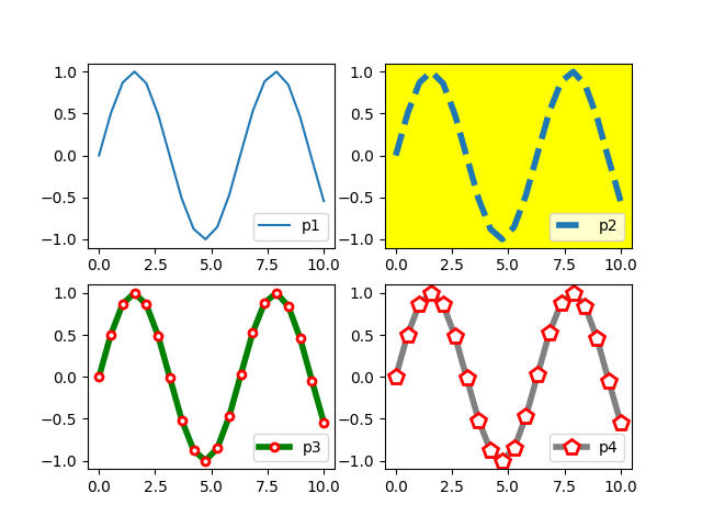
2. 绘制多个图形
x = np.linspace(0, 10, 20)plt.subplot(2,2,1)plt.plot(x, np.sin(x), label='p1')plt.legend(loc=4)plt.subplot(2,2,2, facecolor='yellow')plt.plot(x, np.sin(x), '--', markersize=15, linewidth=4, markerfacecolor='white', markeredgecolor='red', markeredgewidth=2, label='p2')plt.legend(loc=4)plt.subplot(2,2,3)plt.plot(x, np.sin(x), '-o', color='green', markersize=5, linewidth=4, markerfacecolor='white', markeredgecolor='red', markeredgewidth=2, label='p3')plt.legend(loc=4)plt.subplot(2,2,4)plt.plot(x, np.sin(x), '-p', color='gray', markersize=10, linewidth=4, markerfacecolor='white', markeredgecolor='red', markeredgewidth=2, label='p4')plt.legend(loc=4)plt.show()
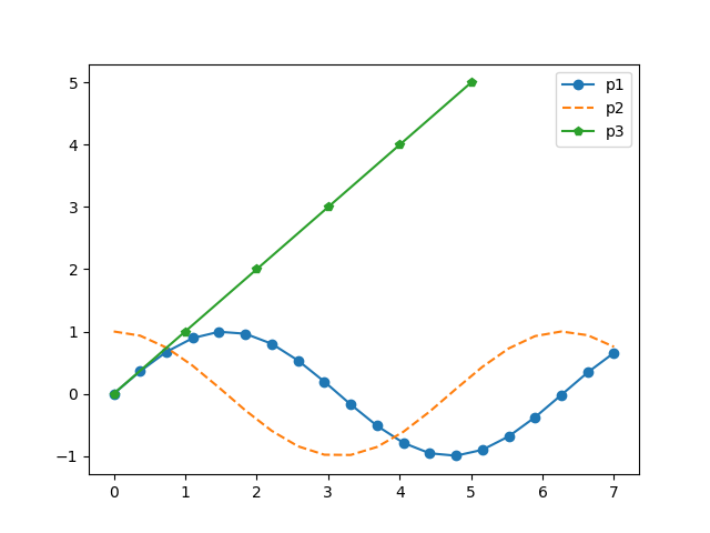
3. 单个图形绘制多条线
x=np.linspace(0, 7, 20)plt.plot(x, np.sin(x), '-o', label='p1')plt.plot(x, np.cos(x), '--', label='p2')plt.plot(range(6), range(6), '-p', label='p3')plt.legend()plt.show()
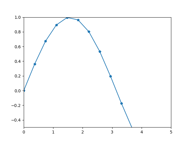
4. ylim、xlim 限定范围绘制图
#ylim、xlim限定范围x=np.linspace(0, 7, 20)plt.plot(x, np.sin(x), '-p')plt.ylim(-0.5, 1)plt.xlim(0, 5)plt.show()
5. 绘制散点图
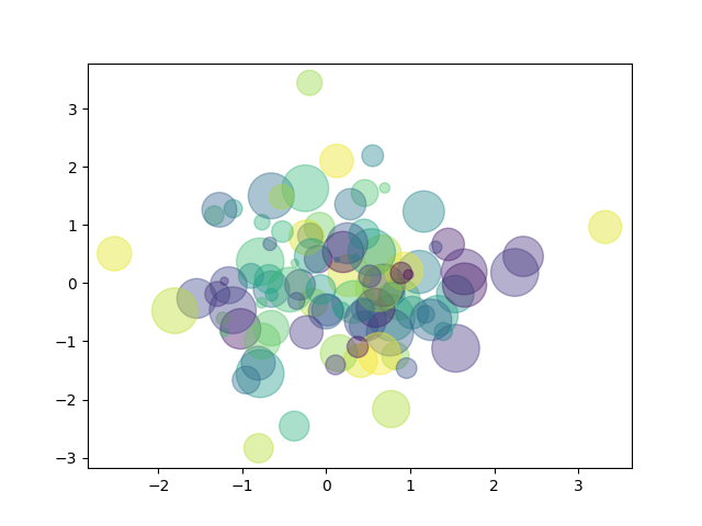
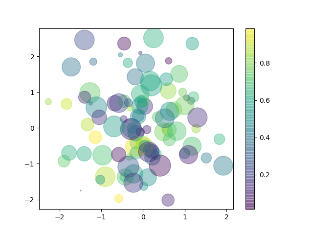
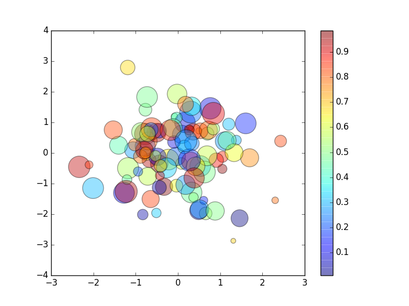
plt.style.use('classic') #设置主题样式, classic经典样式x = np.random.randn(100)y = np.random.randn(100)colors = np.random.rand(100) #0~1之间取值, 生成100个元素的一维数组sizes = 1000 * np.random.rand(100)plt.scatter(x, y, s=sizes, c=colors, alpha=0.4)plt.colorbar()plt.show()
未设经典样式和颜色条,见图4
未设经典样式,见图5
设经典样式和颜色条,见图6
6. 保存绘制的图片
fig = plt.figure()x=np.linspace(0, 7, 20)plt.plot(x, np.sin(x), '-o', label='p1')plt.legend()fig.savefig("/Users/chen/Desktop/python3/project/project1/0-0.png")
2. pandas本身自带制图
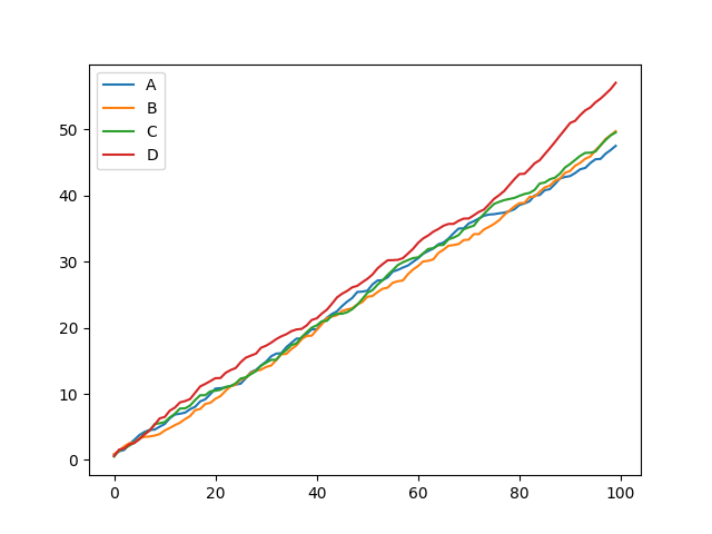
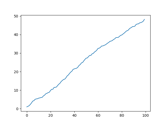
1. 线形图
df = pd.DataFrame(np.random.rand(100, 4).cumsum(0), columns=['A','B','C','D'])df.plot() #整个数组df.A.plot() #某一列plt.show()
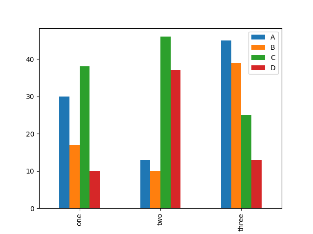
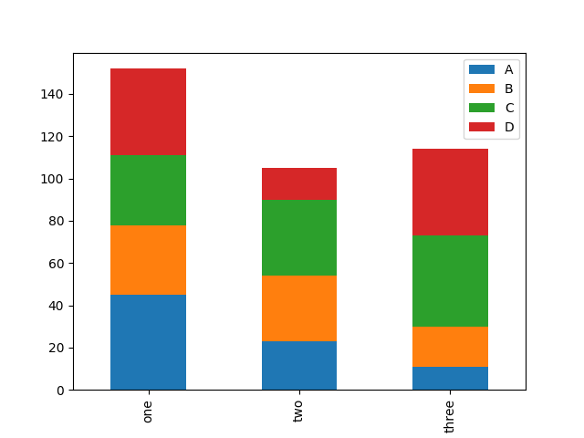
2. 柱状图📊
df = pd.DataFrame(np.random.randint(10, 50, (3,4)), columns=['A', 'B', 'C', 'D'], index=["one", "two", "three"])df.plot(kind='bar', stacked=True) #stacked 叠加df.plot.bar() #整个数组 df.plot.bar() <===> df.plot(kind='bar')df.A.plot.bar() #某一列plt.show()
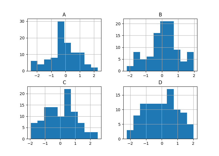
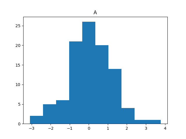
3. 直方图
df = pd.DataFrame(np.random.randn(100, 4), columns=['A','B','C','D'])df.hist()df.hist(column='A', grid=False) #grid:图形的背景网格plt.show()
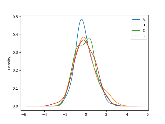
4. 密度图
df = pd.DataFrame(np.random.randn(100, 4), columns=['A','B','C','D'])df.plot.kde()plt.show()