Gmsh tutorial

CFD Gmsh Mesh

1. t1.geo

/*********************************************************************
 *
 *  Gmsh tutorial 1
 *
 *  Variables, elementary entities (points, lines, surfaces), physical
 *  entities (points, lines, surfaces)
 *
 *********************************************************************/
// The simplest construction in Gmsh's scripting language is the
// `affectation'. The following command defines a new variable `lc':
lc = 1e-2;
// This variable can then be used in the definition of Gmsh's simplest
// `elementary entity', a `Point'. A Point is defined by a list of four numbers:
// three coordinates (X, Y and Z), and a characteristic length (lc) that sets
// the target element size at the point:
Point(1) = {0, 0, 0, lc};
// The distribution of the mesh element sizes is then obtained by interpolation
// of these characteristic lengths throughout the geometry. Another method to
// specify characteristic lengths is to use a background mesh (see `t7.geo' and
// `bgmesh.pos').
// We can then define some additional points as well as our first curve.  Curves
// are Gmsh's second type of elementery entities, and, amongst curves, straight
// lines are the simplest. A straight line is defined by a list of point
// numbers. In the commands below, for example, the line 1 starts at point 1 and
// ends at point 2:
Point(2) = {.1, 0,  0, lc} ;
Point(3) = {.1, .3, 0, lc} ;
Point(4) = {0,  .3, 0, lc} ;
Line(1) = {1,2} ;
Line(2) = {3,2} ;
Line(3) = {3,4} ;
Line(4) = {4,1} ;
// The third elementary entity is the surface. In order to define a simple
// rectangular surface from the four lines defined above, a line loop has first
// to be defined. A line loop is a list of connected lines, a sign being
// associated with each line (depending on the orientation of the line):
Line Loop(5) = {4,1,-2,3} ;
// We can then define the surface as a list of line loops (only one here, since
// there are no holes--see `t4.geo'):
Plane Surface(6) = {5} ;
// At this level, Gmsh knows everything to display the rectangular surface 6 and
// to mesh it. An optional step is needed if we want to associate specific
// region numbers to the various elements in the mesh (e.g. to the line segments
// discretizing lines 1 to 4 or to the triangles discretizing surface 6). This
// is achieved by the definition of `physical entities'. Physical entities will
// group elements belonging to several elementary entities by giving them a
// common number (a region number).
// We can for example group the points 1 and 2 into the physical entity 1:
Physical Point(1) = {1,2} ;
// Consequently, two punctual elements will be saved in the output mesh file,
// both with the region number 1. The mechanism is identical for line or surface
// elements:
MY_LINE = 2;
Physical Line(MY_LINE) = {1,2} ;
Physical Line("My second line (automatic physical id)") = {3} ;
Physical Line("My third line (physical id 5)", 5) = {4} ;
Physical Surface("My surface") = {6} ;
// All the line elements created during the meshing of lines 1 and 2 will be
// saved in the output mesh file with the physical id 2. The elements from line
// 3 will be saved in the output mesh file with an automatic physical id,
// associated with the label "My second line (automatic physical id)". The
// elements from line 4 will be saved with physical id 5, associated with the
// label "My third line (physical id 5)". And finally, all the triangular
// elements resulting from the discretization of surface 6 will be given an
// automatic physical id associated with the label "My surface").
// Note that if no physical entities are defined, then all the elements in the
// mesh will be saved "as is", with their default orientation.

2. t2.geo

/*********************************************************************
 *
 *  Gmsh tutorial 2
 *
 *  Includes, geometrical transformations, extruded geometries,
 *  elementary entities (volumes), physical entities (volumes)
 *
 *********************************************************************/
// We first include the previous tutorial file, in order to use it as a basis
// for this one:
Include "t1.geo";
// We can then add new points and lines in the same way as we did in `t1.geo':
Point(5) = {0, .4, 0, lc};
Line(5) = {4, 5};
// But Gmsh also provides tools to tranform (translate, rotate, etc.)
// elementary entities or copies of elementary entities. For example, the point
// 3 can be moved by 0.05 units to the left with:
Translate {-0.05, 0, 0} { Point{3}; }
// The resulting point can also be duplicated and translated by 0.1 along the y
// axis:
Translate {0, 0.1, 0} { Duplicata{ Point{3}; } }
// This command created a new point with an automatically assigned id. This id
// can be obtained using the graphical user interface by hovering the mouse over
// it and looking at the bottom of the graphic window: in this case, the new
// point has id "6". Point 6 can then be used to create new entities, e.g.:
Line(7) = {3, 6};
Line(8) = {6, 5};
Line Loop(10) = {5,-8,-7,3};
Plane Surface(11) = {10};
// Using the graphical user interface to obtain the ids of newly created
// entities can sometimes be cumbersome. It can then be advantageous to use the
// return value of the transformation commands directly. For example, the
// Translate command returns a list containing the ids of the translated
// entities. For example, we can translate copies of the two surfaces 6 and 11
// to the right with the following command:
my_new_surfs[] = Translate {0.12, 0, 0} { Duplicata{ Surface{6, 11}; } };
// my_new_surfs[] (note the square brackets) denotes a list, which in this case
// contains the ids of the two new surfaces (check `Tools->Message console' to
// see the message):
Printf("New surfaces '%g' and '%g'", my_new_surfs[0], my_new_surfs[1]);
// In Gmsh lists use square brackets for their definition (mylist[] = {1,2,3};)
// as well as to access their elements (myotherlist[] = {mylist[0],
// mylist[2]};). Note that list indexing starts at 0.
// Volumes are the fourth type of elementary entities in Gmsh. In the same way
// one defines line loops to build surfaces, one has to define surface loops
// (i.e. `shells') to build volumes. The following volume does not have holes
// and thus consists of a single surface loop:
Point(100) = {0., 0.3, 0.13, lc};  Point(101) = {0.08, 0.3, 0.1, lc};
Point(102) = {0.08, 0.4, 0.1, lc}; Point(103) = {0., 0.4, 0.13, lc};
Line(110) = {4, 100};   Line(111) = {3, 101};
Line(112) = {6, 102};   Line(113) = {5, 103};
Line(114) = {103, 100}; Line(115) = {100, 101};
Line(116) = {101, 102}; Line(117) = {102, 103};
Line Loop(118) = {115, -111, 3, 110};  Plane Surface(119) = {118};
Line Loop(120) = {111, 116, -112, -7}; Plane Surface(121) = {120};
Line Loop(122) = {112, 117, -113, -8}; Plane Surface(123) = {122};
Line Loop(124) = {114, -110, 5, 113};  Plane Surface(125) = {124};
Line Loop(126) = {115, 116, 117, 114}; Plane Surface(127) = {126};
Surface Loop(128) = {127, 119, 121, 123, 125, 11};
Volume(129) = {128};
// When a volume can be extruded from a surface, it is usually easier to use the
// Extrude command directly instead of creating all the points, lines and
// surfaces by hand. For example, the following command extrudes the surface 11
// along the z axis and automatically creates a new volume (as well as all the
// needed points, lines and surfaces):
Extrude {0, 0, 0.12} { Surface{my_new_surfs[1]}; }
// The following command permits to manually assign a characteristic length to
// some of the new points:
Characteristic Length {103, 105, 109, 102, 28, 24, 6, 5} = lc * 3;
// Note that, if the transformation tools are handy to create complex
// geometries, it is also sometimes useful to generate the `flat' geometry, with
// an explicit list of all elementary entities. This can be achieved by
// selecting the `File->Save as->Gmsh unrolled geometry' menu or by typing
//
// > gmsh t2.geo -0
//
// on the command line.
// To save all the tetrahedra discretizing the volumes 129 and 130 with a common
// region number, we finally define a physical volume:
Physical Volume ("The volume", 1) = {129,130};

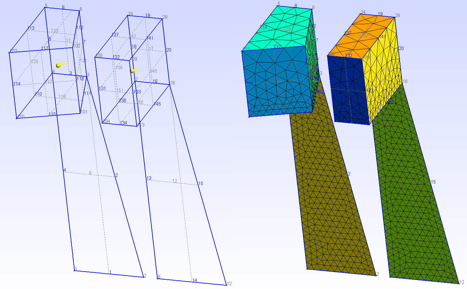
3. t3.geo

/*********************************************************************
 *
 *  Gmsh tutorial 3
 *
 *  Extruded meshes, parameters, options
 *
 *********************************************************************/
Geometry.OldNewReg = 1;
// Again, we start by including the first tutorial:
Include "t1.geo";
// As in `t2.geo', we plan to perform an extrusion along the z axis.  But here,
// instead of only extruding the geometry, we also want to extrude the 2D
// mesh. This is done with the same `Extrude' command, but by specifying element
// 'Layers' (2 layers in this case, the first one with 8 subdivisions and the
// second one with 2 subdivisions, both with a height of h/2):
h = 0.1;
Extrude {0,0,h} {
  Surface{6}; Layers{ {8,2}, {0.5,1} };
}
// The extrusion can also be performed with a rotation instead of a translation,
// and the resulting mesh can be recombined into prisms (we use only one layer
// here, with 7 subdivisions). All rotations are specified by an axis direction
// ({0,1,0}), an axis point ({-0.1,0,0.1}) and a rotation angle (-Pi/2):
Extrude { {0,1,0} , {-0.1,0,0.1} , -Pi/2 } {
  Surface{28}; Layers{7}; Recombine;
}
// Note that a translation ({-2*h,0,0}) and a rotation ({1,0,0}, {0,0.15,0.25},
// Pi/2) can also be combined. Here the angle is specified as a 'parameter',
// using the 'DefineConstant' syntax.  This parameter can be modified
// insteractively in the GUI, and can be exchanged with other codes using the
// ONELAB framework:
DefineConstant[ angle = {90, Min 0, Max 120, Step 1,
                         Name "Parameters/Twisting angle"} ];
out[] = Extrude { {-2*h,0,0}, {1,0,0} , {0,0.15,0.25} , angle * Pi / 180 } {
  Surface{50}; Layers{10}; Recombine;
};
// In this last extrusion command we retrieved the volume number programatically
// by using the return value (a list) of the Extrude command. This list contains
// the "top" of the extruded surface (in out[0]), the newly created volume (in
// out[1]) and the ids of the lateral surfaces (in out[2], out[3], ...)
// We can then define a new physical volume to save all the tetrahedra with a
// common region number (101):
Physical Volume(101) = {1, 2, out[1]};
// Let us now change some options... Since all interactive options are
// accessible in Gmsh's scripting language, we can for example make point tags
// visible or redefine some colors directly in the input file:
Geometry.PointNumbers = 1;
Geometry.Color.Points = Orange;
General.Color.Text = White;
Mesh.Color.Points = {255,0,0};
// Note that all colors can be defined literally or numerically, i.e.
// `Mesh.Color.Points = Red' is equivalent to `Mesh.Color.Points = {255,0,0}';
// and also note that, as with user-defined variables, the options can be used
// either as right or left hand sides, so that the following command will set
// the surface color to the same color as the points:
Geometry.Color.Surfaces = Geometry.Color.Points;
// You can use the `Help->Current options' menu to see the current values of all
// options. To save all the options in a file, use `File->Save as->Gmsh
// options'. To associate the current options with the current file use
// `File->Save Options->For Current File'. To save the current options for all
// future Gmsh sessions use `File->Save Options->As default'.

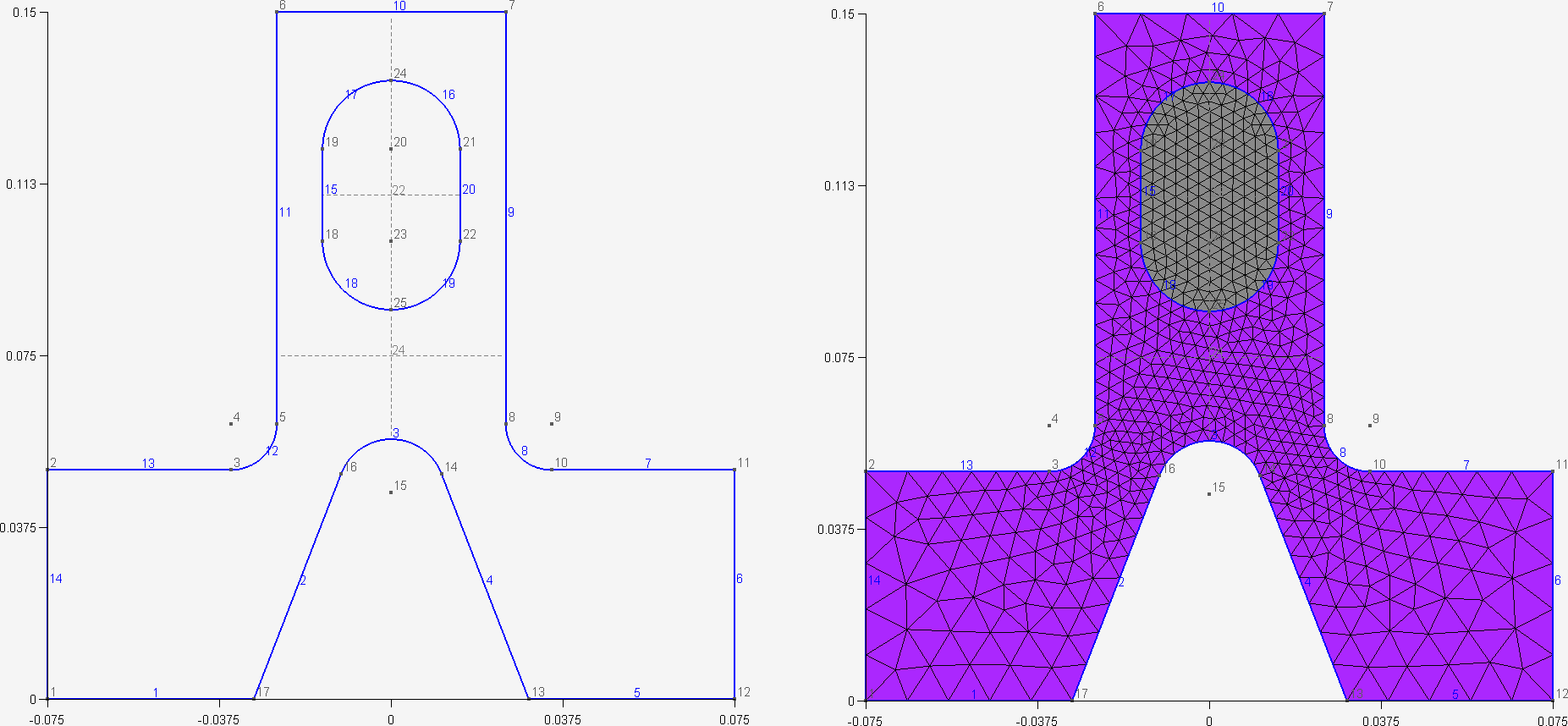
4. t4.geo

/*********************************************************************
 *
 *  Gmsh tutorial 4
 *
 *  Built-in functions, surface holes, annotations, mesh colors
 *
 *********************************************************************/
// As usual, we start by defining some variables:
cm = 1e-02;
e1 = 4.5 * cm; e2 = 6 * cm / 2; e3 =  5 * cm / 2;
h1 = 5 * cm; h2 = 10 * cm; h3 = 5 * cm; h4 = 2 * cm; h5 = 4.5 * cm;
R1 = 1 * cm; R2 = 1.5 * cm; r = 1 * cm;
Lc1 = 0.01;
Lc2 = 0.003;
// We can use all the usual mathematical functions (note the capitalized first
// letters), plus some useful functions like Hypot(a, b) := Sqrt(a^2 + b^2):
ccos = (-h5*R1 + e2 * Hypot(h5, Hypot(e2, R1))) / (h5^2 + e2^2);
ssin = Sqrt(1 - ccos^2);
// Then we define some points and some lines using these variables:
Point(1) = {-e1-e2, 0    , 0, Lc1}; Point(2) = {-e1-e2, h1   , 0, Lc1};
Point(3) = {-e3-r , h1   , 0, Lc2}; Point(4) = {-e3-r , h1+r , 0, Lc2};
Point(5) = {-e3   , h1+r , 0, Lc2}; Point(6) = {-e3   , h1+h2, 0, Lc1};
Point(7) = { e3   , h1+h2, 0, Lc1}; Point(8) = { e3   , h1+r , 0, Lc2};
Point(9) = { e3+r , h1+r , 0, Lc2}; Point(10)= { e3+r , h1   , 0, Lc2};
Point(11)= { e1+e2, h1   , 0, Lc1}; Point(12)= { e1+e2, 0    , 0, Lc1};
Point(13)= { e2   , 0    , 0, Lc1};
Point(14)= { R1 / ssin, h5+R1*ccos, 0, Lc2};
Point(15)= { 0        , h5        , 0, Lc2};
Point(16)= {-R1 / ssin, h5+R1*ccos, 0, Lc2};
Point(17)= {-e2       , 0.0       , 0, Lc1};
Point(18)= {-R2 , h1+h3   , 0, Lc2}; Point(19)= {-R2 , h1+h3+h4, 0, Lc2};
Point(20)= { 0  , h1+h3+h4, 0, Lc2}; Point(21)= { R2 , h1+h3+h4, 0, Lc2};
Point(22)= { R2 , h1+h3   , 0, Lc2}; Point(23)= { 0  , h1+h3   , 0, Lc2};
Point(24)= { 0, h1+h3+h4+R2, 0, Lc2}; Point(25)= { 0, h1+h3-R2,    0, Lc2};
Line(1)  = {1 , 17};
Line(2)  = {17, 16};
// Gmsh provides other curve primitives than stright lines: splines, B-splines,
// circle arcs, ellipse arcs, etc. Here we define a new circle arc, starting at
// point 14 and ending at point 16, with the circle's center being the point 15:
Circle(3) = {14,15,16};
// Note that, in Gmsh, circle arcs should always be smaller than Pi. We can then
// define additional lines and circles, as well as a new surface:
Line(4)  = {14,13}; Line(5)   = {13,12};  Line(6)  = {12,11};
Line(7)  = {11,10}; Circle(8) = {8,9,10}; Line(9)  = {8,7};
Line(10) = {7,6};   Line(11)  = {6,5};    Circle(12) = {3,4,5};
Line(13) = {3,2};   Line(14)  = {2,1};    Line(15) = {18,19};
Circle(16) = {21,20,24}; Circle(17) = {24,20,19};
Circle(18) = {18,23,25}; Circle(19) = {25,23,22};
Line(20) = {21,22};
Line Loop(21) = {17,-15,18,19,-20,16};
Plane Surface(22) = {21};
// But we still need to define the exterior surface. Since this surface has a
// hole, its definition now requires two lines loops:
Line Loop(23) = {11,-12,13,14,1,2,-3,4,5,6,7,-8,9,10};
Plane Surface(24) = {23,21};
// As a general rule, if a surface has N holes, it is defined by N+1 line loops:
// the first loop defines the exterior boundary; the other loops define the
// boundaries of the holes.
// Finally, we can add some comments by embedding a post-processing view
// containing some strings:
View "comments" {
  // Add a text string in window coordinates, 10 pixels from the left and 10
  // pixels from the bottom, using the StrCat function to concatenate strings:
  T2(10, -10, 0){ StrCat("Created on ", Today, " with Gmsh") };
  // Add a text string in model coordinates centered at (X,Y,Z) = (0, 0.11, 0):
  T3(0, 0.11, 0, TextAttributes("Align", "Center", "Font", "Helvetica")){ "Hole" };
  // If a string starts with `file://', the rest is interpreted as an image
  // file. For 3D annotations, the size in model coordinates can be specified
  // after a `@' symbol in the form `widthxheight' (if one of `width' or
  // `height' is zero, natural scaling is used; if both are zero, original image
  // dimensions in pixels are used):
  T3(0, 0.09, 0, TextAttributes("Align", "Center")){ "file://image.png@0.01x0" };
  // The 3D orientation of the image can be specified by proving the direction
  // of the bottom and left edge of the image in model space:
  T3(-0.01, 0.09, 0, 0){ "file://image.png@0.01x0,0,0,1,0,1,0" };
  // The image can also be drawn in "billboard" mode, i.e. always parallel to
  // the camera, by using the `#' symbol:
  T3(0, 0.12, 0, TextAttributes("Align", "Center")){ "file://image.png@0.01x0#" };
  // The size of 2D annotations is given directly in pixels:
  T2(350, -7, 0){ "file://image.png@20x0" };
};
// Views and geometrical entities can be made to respond to double-click events:
View[0].DoubleClickedCommand = "Printf('View[0] has been double-clicked!');";
Geometry.DoubleClickedLineCommand = "Printf('Line %g has been double-clicked!',
  Geometry.DoubleClickedEntityTag);";
// We can also change the color of some mesh entities:
Color Grey50{ Surface{ 22 }; }
Color Purple{ Surface{ 24 }; }
Color Red{ Line{ 1:14 }; }
Color Yellow{ Line{ 15:20 }; }

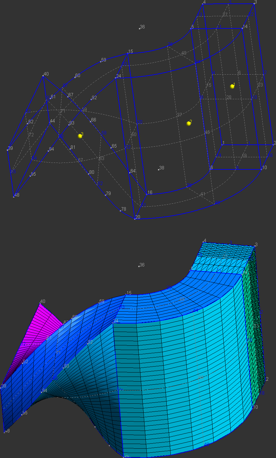
5. t5.geo

/*********************************************************************
 *
 *  Gmsh tutorial 5
 *
 *  Characteristic lengths, arrays of variables, macros, loops
 *
 *********************************************************************/
// We start by defining some target mesh sizes:
lcar1 = .1;
lcar2 = .0005;
lcar3 = .055;
// If we wanted to change these mesh sizes globally (without changing the above
// definitions), we could give a global scaling factor for all characteristic
// lengths on the command line with the `-clscale' option (or with
// `Mesh.CharacteristicLengthFactor' in an option file). For example, with:
//
// > gmsh t5.geo -clscale 1
//
// this input file produces a mesh of approximately 1,300 nodes and 11,000
// tetrahedra. With
//
// > gmsh t5.geo -clscale 0.2
//
// the mesh counts approximately 350,000 nodes and 2.1 million tetrahedra. You
// can check mesh statistics in the graphical user interface with the
// `Tools->Statistics' menu.
// We proceed by defining some elementary entities describing a truncated cube:
Point(1) = {0.5,0.5,0.5,lcar2}; Point(2) = {0.5,0.5,0,lcar1};
Point(3) = {0,0.5,0.5,lcar1};   Point(4) = {0,0,0.5,lcar1};
Point(5) = {0.5,0,0.5,lcar1};   Point(6) = {0.5,0,0,lcar1};
Point(7) = {0,0.5,0,lcar1};     Point(8) = {0,1,0,lcar1};
Point(9) = {1,1,0,lcar1};       Point(10) = {0,0,1,lcar1};
Point(11) = {0,1,1,lcar1};      Point(12) = {1,1,1,lcar1};
Point(13) = {1,0,1,lcar1};      Point(14) = {1,0,0,lcar1};
Line(1) = {8,9};    Line(2) = {9,12};  Line(3) = {12,11};
Line(4) = {11,8};   Line(5) = {9,14};  Line(6) = {14,13};
Line(7) = {13,12};  Line(8) = {11,10}; Line(9) = {10,13};
Line(10) = {10,4};  Line(11) = {4,5};  Line(12) = {5,6};
Line(13) = {6,2};   Line(14) = {2,1};  Line(15) = {1,3};
Line(16) = {3,7};   Line(17) = {7,2};  Line(18) = {3,4};
Line(19) = {5,1};   Line(20) = {7,8};  Line(21) = {6,14};
Line Loop(22) = {-11,-19,-15,-18};   Plane Surface(23) = {22};
Line Loop(24) = {16,17,14,15};       Plane Surface(25) = {24};
Line Loop(26) = {-17,20,1,5,-21,13}; Plane Surface(27) = {26};
Line Loop(28) = {-4,-1,-2,-3};       Plane Surface(29) = {28};
Line Loop(30) = {-7,2,-5,-6};        Plane Surface(31) = {30};
Line Loop(32) = {6,-9,10,11,12,21};  Plane Surface(33) = {32};
Line Loop(34) = {7,3,8,9};           Plane Surface(35) = {34};
Line Loop(36) = {-10,18,-16,-20,4,-8}; Plane Surface(37) = {36};
Line Loop(38) = {-14,-13,-12,19};    Plane Surface(39) = {38};
// Instead of using included files, we now use a user-defined macro in order
// to carve some holes in the cube:
Macro CheeseHole
  // In the following commands we use the reserved variable name `newp', which
  // automatically selects a new point number. This number is chosen as the
  // highest current point number, plus one. (Note that, analogously to `newp',
  // the variables `newl', `news', `newv' and `newreg' select the highest number
  // amongst currently defined curves, surfaces, volumes and `any entities other
  // than points', respectively.)
  p1 = newp; Point(p1) = {x,  y,  z,  lcar3} ;
  p2 = newp; Point(p2) = {x+r,y,  z,  lcar3} ;
  p3 = newp; Point(p3) = {x,  y+r,z,  lcar3} ;
  p4 = newp; Point(p4) = {x,  y,  z+r,lcar3} ;
  p5 = newp; Point(p5) = {x-r,y,  z,  lcar3} ;
  p6 = newp; Point(p6) = {x,  y-r,z,  lcar3} ;
  p7 = newp; Point(p7) = {x,  y,  z-r,lcar3} ;
  c1 = newreg; Circle(c1) = {p2,p1,p7}; c2 = newreg; Circle(c2) = {p7,p1,p5};
  c3 = newreg; Circle(c3) = {p5,p1,p4}; c4 = newreg; Circle(c4) = {p4,p1,p2};
  c5 = newreg; Circle(c5) = {p2,p1,p3}; c6 = newreg; Circle(c6) = {p3,p1,p5};
  c7 = newreg; Circle(c7) = {p5,p1,p6}; c8 = newreg; Circle(c8) = {p6,p1,p2};
  c9 = newreg; Circle(c9) = {p7,p1,p3}; c10 = newreg; Circle(c10) = {p3,p1,p4};
  c11 = newreg; Circle(c11) = {p4,p1,p6}; c12 = newreg; Circle(c12) = {p6,p1,p7};
  // We need non-plane surfaces to define the spherical holes. Here we use ruled
  // surfaces, which can have 3 or 4 sides:
  l1 = newreg; Line Loop(l1) = {c5,c10,c4};   Ruled Surface(newreg) = {l1};
  l2 = newreg; Line Loop(l2) = {c9,-c5,c1};   Ruled Surface(newreg) = {l2};
  l3 = newreg; Line Loop(l3) = {c12,-c8,-c1}; Ruled Surface(newreg) = {l3};
  l4 = newreg; Line Loop(l4) = {c8,-c4,c11};  Ruled Surface(newreg) = {l4};
  l5 = newreg; Line Loop(l5) = {-c10,c6,c3};  Ruled Surface(newreg) = {l5};
  l6 = newreg; Line Loop(l6) = {-c11,-c3,c7}; Ruled Surface(newreg) = {l6};
  l7 = newreg; Line Loop(l7) = {-c2,-c7,-c12};Ruled Surface(newreg) = {l7};
  l8 = newreg; Line Loop(l8) = {-c6,-c9,c2};  Ruled Surface(newreg) = {l8};
  // We then store the surface loops identification numbers in a list for later
  // reference (we will need these to define the final volume):
  theloops[t] = newreg ;
  Surface Loop(theloops[t]) = {l8+1,l5+1,l1+1,l2+1,l3+1,l7+1,l6+1,l4+1};
  thehole = newreg ;
  Volume(thehole) = theloops[t] ;
Return
// We can use a `For' loop to generate five holes in the cube:
x = 0 ; y = 0.75 ; z = 0 ; r = 0.09 ;
For t In {1:5}
  x += 0.166 ;
  z += 0.166 ;
  // We call the `CheeseHole' macro:
  Call CheeseHole ;
  // We define a physical volume for each hole:
  Physical Volume (t) = thehole ;
  // We also print some variables on the terminal (note that, since all
  // variables are treated internally as floating point numbers, the format
  // string should only contain valid floating point format specifiers like
  // `%g', `%f', '%e', etc.):
  Printf("Hole %g (center = {%g,%g,%g}, radius = %g) has number %g!",
     t, x, y, z, r, thehole) ;
EndFor
// We can then define the surface loop for the exterior surface of the cube:
theloops[0] = newreg ;
Surface Loop(theloops[0]) = {35,31,29,37,33,23,39,25,27} ;
// The volume of the cube, without the 5 holes, is now defined by 6 surface
// loops: the first surface loop defines the exterior surface; the surface loops
// other than the first one define holes.  (Again, to reference an array of
// variables, its identifier is followed by square brackets):
Volume(186) = {theloops[]} ;
// We finally define a physical volume for the elements discretizing the cube,
// without the holes (whose elements were already tagged with numbers 1 to 5 in
// the `For' loop):
Physical Volume (10) = 186 ;
// We could make only part of the model visible to only mesh this subset:
//
// Hide "*";
// Recursive Show { Volume{129}; }
// Mesh.MeshOnlyVisible=1;

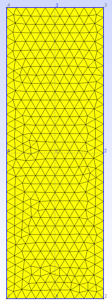
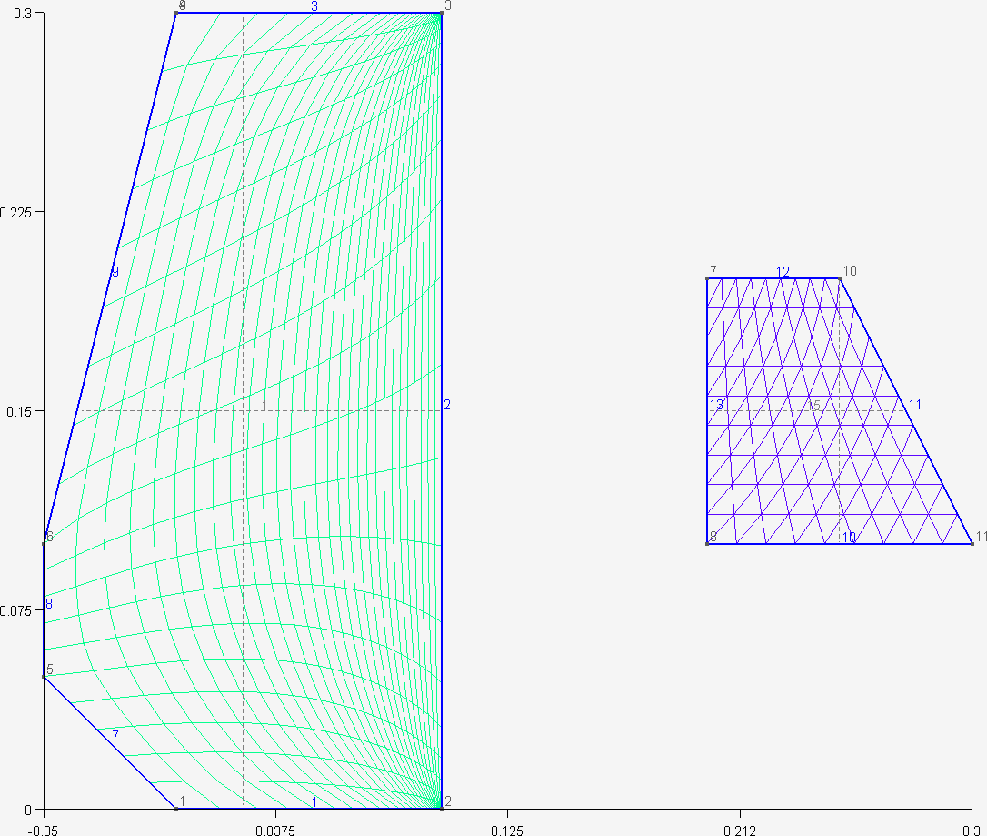
6. t6.geo

/*********************************************************************
 *
 *  Gmsh tutorial 6
 *
 *  Transfinite meshes
 *
 *********************************************************************/
// Let's use the geometry from the first tutorial as a basis for this one
Include "t1.geo";
// Delete the left line and create replace it with 3 new ones
Delete{ Surface{6}; Line{4}; }
p1 = newp; Point(p1) = {-0.05, 0.05, 0, lc};
p2 = newp; Point(p2) = {-0.05, 0.1, 0, lc};
l1 = newl; Line(l1) = {1, p1};
l2 = newl; Line(l2) = {p1, p2};
l3 = newl; Line(l3) = {p2, 4};
// Create surface
Line Loop(1) = {2, -1, l1, l2, l3, -3};
Plane Surface(1) = {-1};
// Put 20 points with a refinement toward the extremities on curve 2
Transfinite Line{2} = 20 Using Bump 0.05;
// Put 20 points total on combination of curves l1, l2 and l3 (beware that the
// points p1 and p2 are shared by the curves, so we do not create 6 + 6 + 10 =
// 22 points, but 20!)
Transfinite Line{l1} = 6;
Transfinite Line{l2} = 6;
Transfinite Line{l3} = 10;
// Put 30 points following a geometric progression on curve 1 (reversed) and on
// curve 3
Transfinite Line{-1,3} = 30 Using Progression 1.2;
// Define the Surface as transfinite, by specifying the four corners of the
// transfinite interpolation
Transfinite Surface{1} = {1,2,3,4};
// (Note that the list on the right hand side refers to points, not curves. When
// the surface has only 3 or 4 points on its boundary the list can be
// omitted. The way triangles are generated can be controlled by appending
// "Left", "Right" or "Alternate" after the list.)
// Recombine the triangles into quads
Recombine Surface{1};
// Apply an elliptic smoother to the grid
Mesh.Smoothing = 100;
Physical Surface(1) = 1;
// When the surface has only 3 or 4 control points, the transfinite constraint
// can be applied automatically (without specifying the corners explictly).
Point(7) = {0.2, 0.2, 0, 1.0};
Point(8) = {0.2, 0.1, 0, 1.0};
Point(9) = {-0, 0.3, 0, 1.0};
Point(10) = {0.25, 0.2, 0, 1.0};
Point(11) = {0.3, 0.1, 0, 1.0};
Line(10) = {8, 11};
Line(11) = {11, 10};
Line(12) = {10, 7};
Line(13) = {7, 8};
Line Loop(14) = {13, 10, 11, 12};
Plane Surface(15) = {14};
Transfinite Line {10:13} = 10;
Transfinite Surface{15};

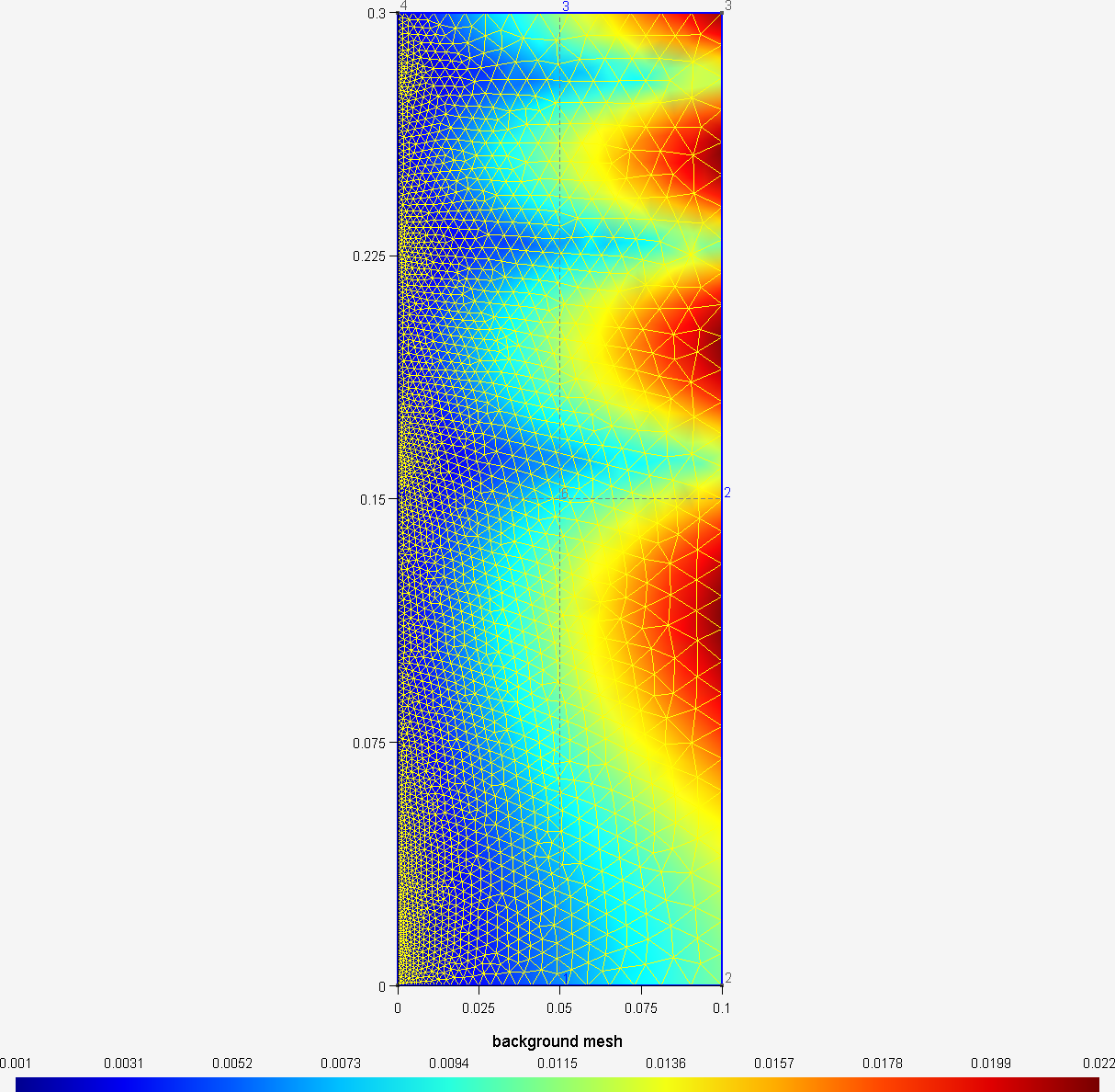
7. t7.geo

/*********************************************************************
 *
 *  Gmsh tutorial 7
 *
 *  Background mesh
 *
 *********************************************************************/
// Characteristic lengths can be specified very accuractely by providing a
// background mesh, i.e., a post-processing view that contains the target mesh
// sizes.
// Merge the first tutorial
Merge "t1.geo";
// Merge a post-processing view containing the target mesh sizes
Merge "bgmesh.pos";
// Apply the view as the current background mesh
Background Mesh View[0];

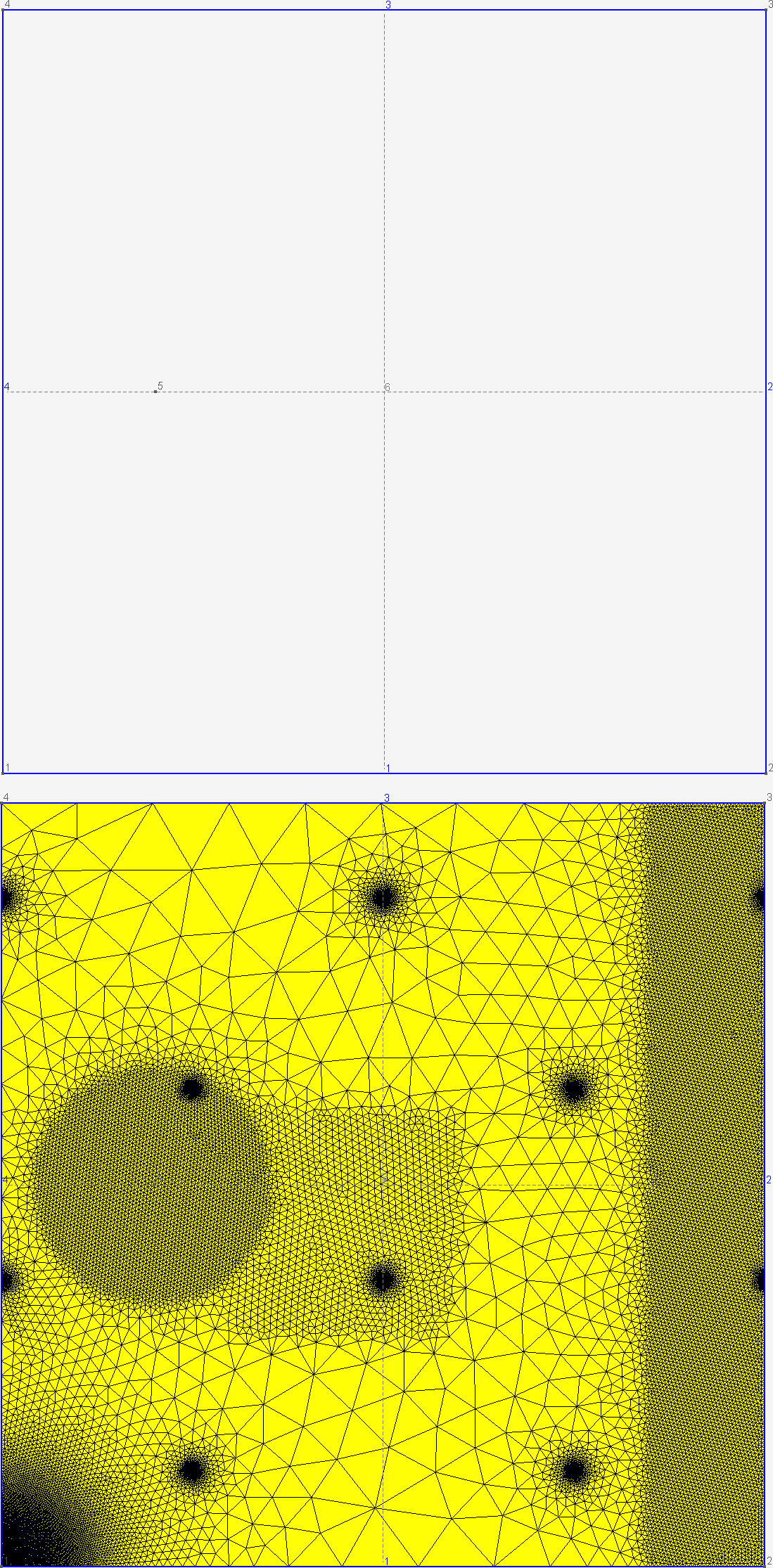
10. t10.geo

/*********************************************************************
 *
 *  Gmsh tutorial 10
 *
 *  General mesh size fields
 *
 *********************************************************************/
// In addition to specifying target mesh sizes at the points of the
// geometry (see t1) or using a background mesh (see t7), you can use
// general mesh size "Fields".
// Let's create a simple rectangular geometry
lc = .15;
Point(1) = {0.0,0.0,0,lc}; Point(2) = {1,0.0,0,lc};
Point(3) = {1,1,0,lc};     Point(4) = {0,1,0,lc};
Point(5) = {0.2,.5,0,lc};
Line(1) = {1,2}; Line(2) = {2,3}; Line(3) = {3,4}; Line(4) = {4,1};
Line Loop(5) = {1,2,3,4}; Plane Surface(6) = {5};
// Say we would like to obtain mesh elements with size lc/30 near line 1 and
// point 5, and size lc elsewhere. To achieve this, we can use two fields:
// "Attractor", and "Threshold". We first define an Attractor field (Field[1])
// on points 5 and on line 1. This field returns the distance to point 5 and to
// (100 equidistant points on) line 1.
Field[1] = Attractor;
Field[1].NodesList = {5};
Field[1].NNodesByEdge = 100;
Field[1].EdgesList = {2};
// We then define a Threshold field, which uses the return value of the
// Attractor Field[1] in order to define a simple change in element size around
// the attractors (i.e., around point 5 and line 1)
//
// LcMax -                         /------------------
//                               /
//                             /
//                           /
// LcMin -o----------------/
//        |                |       |
//     Attractor       DistMin   DistMax
Field[2] = Threshold;
Field[2].IField = 1;
Field[2].LcMin = lc / 30;
Field[2].LcMax = lc;
Field[2].DistMin = 0.15;
Field[2].DistMax = 0.5;
// Say we want to modulate the mesh element sizes using a mathematical function
// of the spatial coordinates. We can do this with the MathEval field:
Field[3] = MathEval;
Field[3].F = "Cos(4*3.14*x) * Sin(4*3.14*y) / 10 + 0.101";
// We could also combine MathEval with values coming from other fields. For
// example, let's define an Attractor around point 1
Field[4] = Attractor;
Field[4].NodesList = {1};
// We can then create a MathEval field with a function that depends on the
// return value of the Attractr Field[4], i.e., depending on the distance to
// point 1 (here using a cubic law, with minumum element size = lc / 100)
Field[5] = MathEval;
Field[5].F = Sprintf("F4^3 + %g", lc / 100);
// We could also use a Box field to impose a step change in element sizes inside
// a box
Field[6] = Box;
Field[6].VIn = lc / 15;
Field[6].VOut = lc;
Field[6].XMin = 0.3;
Field[6].XMax = 0.6;
Field[6].YMin = 0.3;
Field[6].YMax = 0.6;
// Many other types of fields are available: see the reference manual for a
// complete list. You can also create fields directly in the graphical user
// interface by selecting Define->Fields in the Mesh module.
// Finally, let's use the minimum of all the fields as the background mesh field
Field[7] = Min;
Field[7].FieldsList = {2, 3, 5, 6};
Background Field = 7;
// If the boundary mesh size was too small, we could ask not to extend the
// elements sizes from the boundary inside the domain:
// Mesh.CharacteristicLengthExtendFromBoundary = 0;

x. t[x].geo

to be continued...