Exercise_5:The Trajectory of a cannon shell

physics python

Abstract

• I plan to choose problem_2.6 to make a practice.

Use the Euler method to calculate cannon shell trajectories ignoring both air drag and the effect of air density(actually, ignoring the former automatically rules out the latter). Compare your results with those in Figure 2.4, and with the exact solution.

Background

The Euler method we used to treat the bicycle problem can easily be generalized to deal with motion in two spatial dimensions. To be specific, we consider a projectile such as a shell shot by a cannon. We have a very large cannon in mind, and the large size will determine some of the important physics...

Main

Exercise_2.6

Use the Euler method to calculate cannon shell trajectories ignoring both air drag and the effect of air density(actually, ignoring the former automatically rules out the latter). Compare your results with those in Figure 2.4, and with the exact solution.

Solution

• Subroutine calculate for the cannon shell projectile using the Euler Method

• Store position as $(x_i,y_i)$ and velocity as $(v_{x,i},v_{y,i})$.

• For each time step $i$ calculate position and velocity at step $i+1$:

$$x_{i+1}=x_i+v_{x,i}\Delta{t}$$

$$v_{x,i+1}=v_{x,i}$$

$$y_{i+1}=y_i+v_{y,i}\Delta{t}$$

$$v_{y,i+1}=v_{y+i}-g\Delta{t}$$

• Stop when $y_{i+1}\le0$ or $t\le t_{max}$

• We choose seven lines to show the different trajectors of the cannon shell by using loop statement while.

Codes

import pylab as pl
import math as mt
class cannon_shells:
    def __init__(self, initial_velocity = 0.7, g = 0.0098, range = 0, height = 0,\
                 time_step = 0.01, initial_angle = 30.0, da = 5.0):
        self.v = [initial_velocity]
        self.a = [initial_angle]
        self.g = g
        self.dt = time_step
        self.da = da
        self.x = [range]
        self.y = [height]
    def run(self):
        _a = self.a[0]
        while(_a <= 60):
            _a += self.da
            self.a.append(self.a[-1] + self.da)
            t = 2 * mt.sin(_a / 180.0 * mt.pi) * self.v[0]/self.g
            vx = mt.cos(_a / 180.0 * mt.pi) * self.v[0]
            vy = mt.sin(_a / 180.0 * mt.pi) * self.v[0]
            _time = 0
            xi = [0]
            yi = [0]
            while(_time < t):
                xi.append(xi[-1] + self.dt * vx)
                yi.append(yi[-1] + self.dt * vy)
                vx = vx
                vy = vy - self.g * self.dt
                _time += self.dt
            self.x = self.x + xi
            self.y = self.y + yi
    def show_results(self):
        font = {'family': 'serif',
                'color':  'darkred',
                'weight': 'normal',
                'size': 16,
        }
        pl.title('The trajectory of a cannon shell')
        pl.text(0.95 * self.x[-1], 0.95 * max(self.y),\
                'No drag', fontdict=font)
        pl.plot(self.x,self.y)
        pl.xlabel('x($km$)')
        pl.ylabel('y($km$)')
        pl.show()
a = cannon_shells()
a.run()
a.show_results()

• Running result:

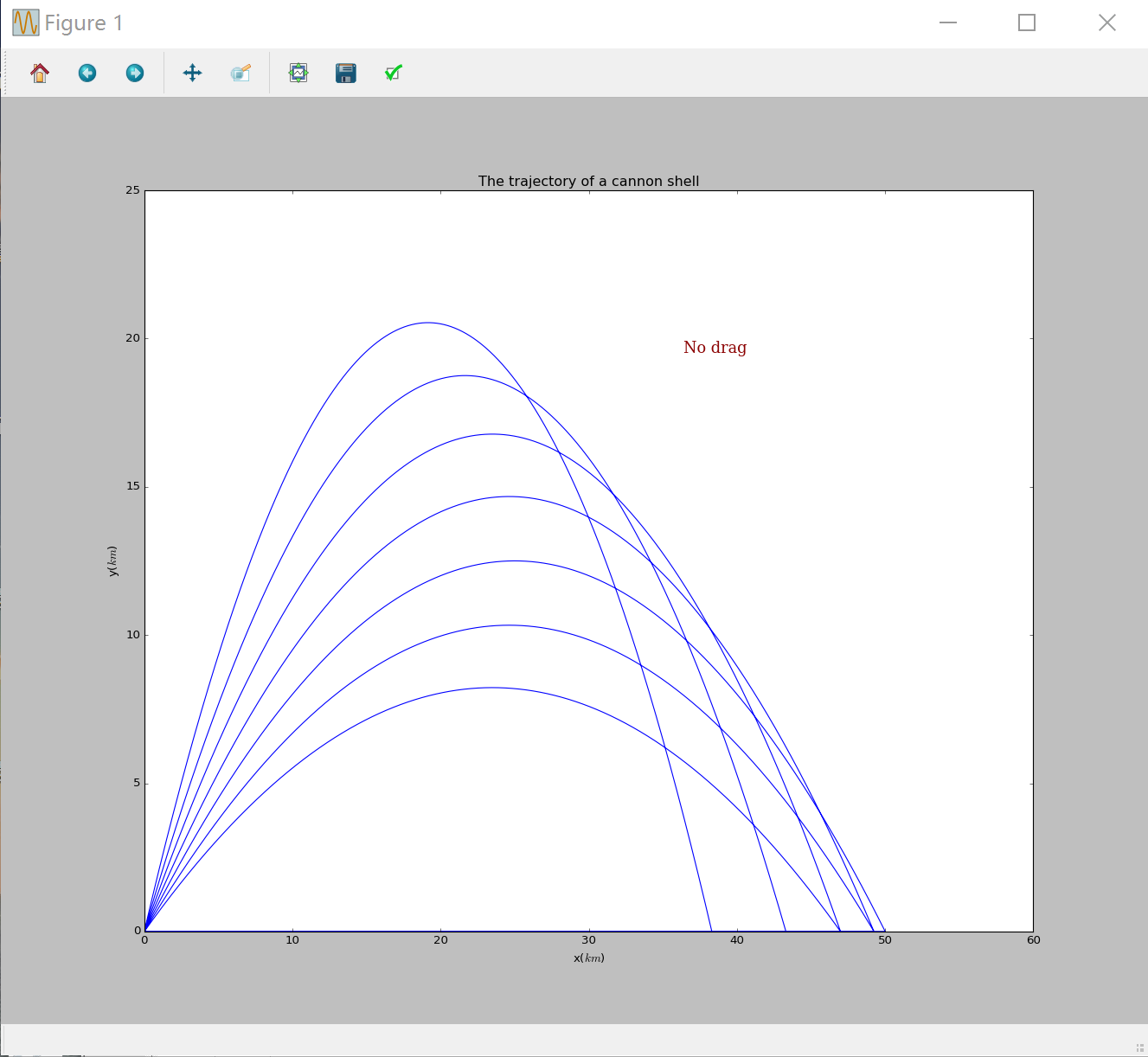
Conclusion

• The results are the same as those in Figure 2.4.

• This is a exact solution.

Acknowledgment

Lesson plan of Cai Hao:Chapter 2