Exercise 10 : Precession of the Perihelion of Mercury

python physics

---

Abstract

In the present chapter we will consider several problems that arise in the study of plantary motion. We begin with the simplest situation, a sun and a single planet, and investigate a few of the properties of this model solar system. While a computational approach is not required in this case, the algorithm we develop will prove useful for later problems. Additionally, comparisions of the numerical results obtained with this algorithm with exact solutions will provide valuable insight into the nature of our approximations.

---

Background

Kepler's Laws

• According to the Newton's law of the gravitation the magnitude of this force is given by
  

  $$F_G=\frac{GM_SM_E}{r^2}$$

• From the Newton's secnd law, we have
  

  $$\frac{d^2x}{dt^2}=\frac{F_{G,x}}{M_E}$$ $$\frac{d^2y}{dt^2}=\frac{F_{G,y}}{M_E}$$

• Thus
  

  $$F_{G,x}=-\frac{GM_SM_E}{r^2}cos\theta=-\frac{GM_SM_Ex}{r^2}$$

• can follow our usual approach and write each of the second-order differential equations as two first-order differential equations.
  

  $$\frac{dv_y}{dt}=-\frac{GM_Sy}{r^3} \frac{dx}{dt}=v_x$$

$$\frac{dv_y}{dt}=-\frac{GM_Sy}{r^3} \frac{dy}{dt}=v_y$$

• We can use Euler-Cromer method to solve the equations:
  $$r_i=(x_i^2+y_i^2)^{1/2}$$

$$v_{x,i+1}=v_{x,i}-\frac{4\pi^2x_i}{r_i^3}\Delta{t}$$

$$x_{i+1}=x_i+v_{x,i+1}\Delta{t}$$

$$v_{y,i+1}=v_{y,i}-\frac{4\pi^2y_i}{r_i^3}\Delta{t}$$

$$y_{i+1}=y_i+v_{y,i+1}\Delta{t}$$

• The orbital trajectory for a body of reduced mass $\mu$ is given in polar coordinates by
  

  $$\frac{d^2}{d\theta^2}(\frac{1}{r})+\frac{1}{r}=-\frac{\mu{r}^2}{L^2}F(r)$$

• Also the momentum L is a constant,
  Thus we have

$$v_{max}=\sqrt{GM_S}\sqrt{\frac{1+e}{a(1-e)}(1+\frac{M_P}{M_S})}$$

$$v_{min}=\sqrt{GM_S}\sqrt{\frac{1-e}{a(1+e)}(1+\frac{M_P}{M_S})}$$

---

Main Body

Problem4.10 Calculate the precession of the perihelion of Mercury, following the approach described in this section.

(Problem4.11)

• Code

import math
import matplotlib.pyplot as plt
GM=4*(math.pi**2)
perihelion=0.39*(1-0.206)
class Precession:
    def __init__(self,e=0.206,time=1,dt=0.0001,vcoefficient=1.1,beta=2.1,alpha=0.01):
        self.alpha=alpha
        self.beta=beta
        self.vcoefficient=vcoefficient
        self.e=e
        self.a=perihelion/(1-e)
        self.x0=self.a*(1+e)
        #self.x0=1
        self.y0=0
        self.vx0=0
        self.vy0=self.vcoefficient*math.sqrt((GM*(1-self.e))/(self.a*(1+self.e)))
        #self.vy0=2*math.pi
        self.X=[self.x0]
        self.Y=[self.y0]
        self.Vx=[self.vx0]
        self.Vy=[self.vy0]
        self.T=[0]
        self.dt=dt
        self.time=time
        self.ThetaPrecession=[]
        self.TimePrecession=[]
    def run(self):
        while self.T[-1]<self.time:
            r=math.sqrt(self.X[-1]**2+self.Y[-1]**2)
            newVx=self.Vx[-1]-(GM*(1+self.alpha/r**2)*self.X[-1]/r**(1+self.beta))*self.dt
            newX=self.X[-1]+newVx*self.dt
            newVy=self.Vy[-1]-(GM*(1+self.alpha/r**2)*self.Y[-1]/r**(1+self.beta))*self.dt
            newY=self.Y[-1]+newVy*self.dt
            if abs(newX*newVx+newY*newVy)<0.0014 and r<self.a:
                theta=math.acos(self.X[-1]/r)*180/math.pi
                if (self.Y[-1]/r)<0:
                    theta=360-theta
                theta=abs(theta-180)
                self.ThetaPrecession.append(theta)
                self.TimePrecession.append(self.T[-1])
            self.Vx.append(newVx)
            self.Vy.append(newVy)
            self.X.append(newX)
            self.Y.append(newY)
            self.T.append(self.T[-1]+self.dt)
    def show_results(self):
        plt.plot(self.X,self.Y,'g')
        plt.legend(loc='upper right',frameon=False,fontsize='small')
        plt.grid(True)
        plt.title('Simulation of the precession of Mercury')
        plt.xlabel('x(AU)')
        plt.ylabel('y(AU)')
        ax = plt.gca()
        ax.set_aspect(1)
        #plt.xlim(-1,1)
        #plt.ylim(-0.6,0.6)
        #plt.scatter(0,0)
A = Precession()
A.run()
A.show_results()

• Result

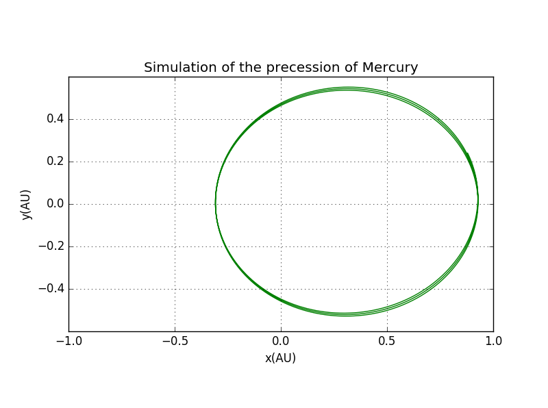
• We can plot the Precession of the Perihelion of Mercury.

• First, we can chose that $\alpha=0.0008,\beta=2,e=0.206$

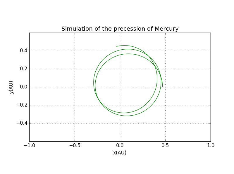
• we can chose different e when $\alpha=0.0008,\beta=2$

Then we can chose a different $\alpha$ to do the work again.
we chose $\alpha=0.01,\beta=2,e=0.206$

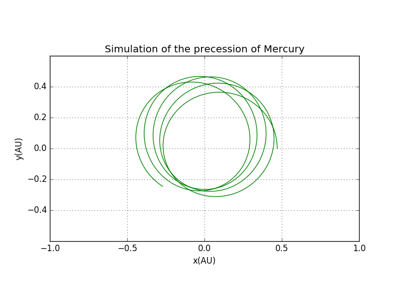
Then we can choose $\alpha=0.1,\beta=2.01$

---

Conclusion

With the help of Kepler's Laws and the Euler-Cromer method, we can solve the motion of the simplest situation where a sun and a single planet get moved with interaction. And we can try to plot the figure of the precession of perihelion of Mercury.

---

Acknowledgment

• peiyu