@BruceWang
2018-01-03T09:16:36.000000Z
字数 10943
阅读 1959
Jupter numpy pandas matplot 笔记
This is my first jupyter notes
NumpyPandasMatplot
1+2
3
def f(x,y,z):return (x+y)/za = 5b=6c=7.5
import numpy as npdata = np.random.rand(2,11)print(data)
[[ 0.67577294  0.194396    0.5525098   0.04609985  0.14534381  0.93533033
   0.32043392  0.0807357   0.46490533  0.89414549  0.260932  ]
 [ 0.78801884  0.25585532  0.99597803  0.09019288  0.58768134  0.0815639
   0.18691377  0.60306836  0.80131033  0.63986103  0.2780275 ]]
type(data), data.shape
(numpy.ndarray, (2, 11))
data.dtype
dtype('float64')
data.dtype
dtype('float64')
second part
data1 = [23,3,4.45,5,3,5,0]
arr1 = np.array(data1)
arr1
array([ 23. , 3. , 4.45, 5. , 3. , 5. , 0. ])
arr1.shapearr1.reshape(1,7)arr1.shape
(7,)
arr1.dtype
dtype('float64')
np.zeros(10)
array([ 0., 0., 0., 0., 0., 0., 0., 0., 0., 0.])
np.zeros((3,4))
array([[ 0.,  0.,  0.,  0.],
       [ 0.,  0.,  0.,  0.],
       [ 0.,  0.,  0.,  0.]])
a = _
a.shape
(3, 4)
np.empty((2,3))
array([[ 23.  ,   3.  ,   4.45],
       [  5.  ,   3.  ,   5.  ]])
np.empty((3,4,5))
array([[[  1.00999541e-311,   1.00997906e-311,   1.00997961e-311,
           1.00997851e-311,   1.00997844e-311],
        [  1.00997838e-311,   1.00997751e-311,   1.00997963e-311,
           1.00997838e-311,   1.00997751e-311],
        [  1.00997768e-311,   1.00997961e-311,   1.00997758e-311,
           1.00997758e-311,   1.00997768e-311],
        [  1.00997758e-311,   1.00997967e-311,   1.00997939e-311,
           1.00997961e-311,   1.00997751e-311]],

       [[  1.00997846e-311,   1.00997865e-311,   1.00997766e-311,
           1.00997838e-311,   1.00997751e-311],
        [  1.00997768e-311,   1.00997865e-311,   1.00997852e-311,
           1.00997838e-311,   1.00997758e-311],
        [  1.00997758e-311,   1.00997838e-311,   1.00997852e-311,
           1.00997865e-311,   1.00997766e-311],
        [  1.00997766e-311,   1.00997865e-311,   1.00997766e-311,
           1.00997768e-311,   1.00997766e-311]],

       [[  1.00997865e-311,   1.00997768e-311,   1.00997768e-311,
           1.00997749e-311,   1.00997766e-311],
        [  1.00997766e-311,   1.00997768e-311,   1.00997768e-311,
           1.00997963e-311,   1.00997963e-311],
        [  1.00997963e-311,   9.21088093e-315,   1.00997964e-311,
           9.21088710e-315,   1.00997964e-311],
        [  9.21088093e-315,   9.21088093e-315,   1.00997962e-311,
           1.00997963e-311,   9.21088093e-315]]])
a = _print(a.shape)print(a)
(3, 4, 5)
[[[  1.00999541e-311   1.00997906e-311   1.00997961e-311   1.00997851e-311
     1.00997844e-311]
  [  1.00997838e-311   1.00997751e-311   1.00997963e-311   1.00997838e-311
     1.00997751e-311]
  [  1.00997768e-311   1.00997961e-311   1.00997758e-311   1.00997758e-311
     1.00997768e-311]
  [  1.00997758e-311   1.00997967e-311   1.00997939e-311   1.00997961e-311
     1.00997751e-311]]

 [[  1.00997846e-311   1.00997865e-311   1.00997766e-311   1.00997838e-311
     1.00997751e-311]
  [  1.00997768e-311   1.00997865e-311   1.00997852e-311   1.00997838e-311
     1.00997758e-311]
  [  1.00997758e-311   1.00997838e-311   1.00997852e-311   1.00997865e-311
     1.00997766e-311]
  [  1.00997766e-311   1.00997865e-311   1.00997766e-311   1.00997768e-311
     1.00997766e-311]]

 [[  1.00997865e-311   1.00997768e-311   1.00997768e-311   1.00997749e-311
     1.00997766e-311]
  [  1.00997766e-311   1.00997768e-311   1.00997768e-311   1.00997963e-311
     1.00997963e-311]
  [  1.00997963e-311   9.21088093e-315   1.00997964e-311   9.21088710e-315
     1.00997964e-311]
  [  9.21088093e-315   9.21088093e-315   1.00997962e-311   1.00997963e-311
     9.21088093e-315]]]
np.arange(21)
array([ 0,  1,  2,  3,  4,  5,  6,  7,  8,  9, 10, 11, 12, 13, 14, 15, 16,
       17, 18, 19, 20])
np.arange(21)
array([ 0,  1,  2,  3,  4,  5,  6,  7,  8,  9, 10, 11, 12, 13, 14, 15, 16,
       17, 18, 19, 20])
array: 将数据转化成ndarray
asarray:将数据转换成ndarray
arange:产生的是一个ndarray,而array产生的是list
arr1 = np.arange(12, dtype=np.float64)print(arr1)
[ 0. 1. 2. 3. 4. 5. 6. 7. 8. 9. 10. 11.]
print(arr1.dtype)type(arr1)
float64


numpy.ndarray
np.arange(12,dtype=np.float64)
array([  0.,   1.,   2.,   3.,   4.,   5.,   6.,   7.,   8.,   9.,  10.,
        11.])
np.eye(5)
array([[ 1.,  0.,  0.,  0.,  0.],
       [ 0.,  1.,  0.,  0.,  0.],
       [ 0.,  0.,  1.,  0.,  0.],
       [ 0.,  0.,  0.,  1.,  0.],
       [ 0.,  0.,  0.,  0.,  1.]])
向量化的数组运算比纯python同等程度的运算要快很多。
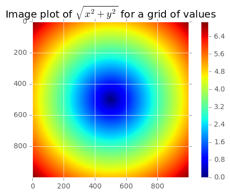
一个简单的例子,假设我们想要评价函数sqrt(x^2 + y^2)
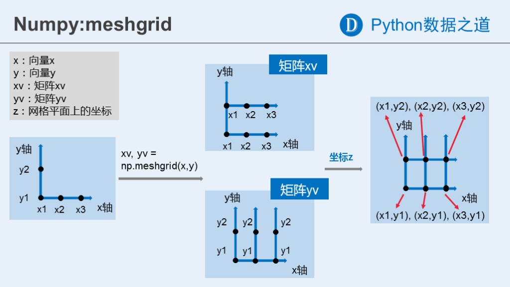
np.meshgrid函数取两个1维的数组,产生一个2位的矩阵,对应于所有两个数组中(x, y)的组合:
import numpy as np
在进行书中的内容之前,先举个例子说明meshgrid的效果。meshgrid函数用两个坐标轴上的点在平面上画网格。
用法:
- [X,Y]=meshgrid(x,y)
- [X,Y]=meshgrid(x)与[X,Y]=meshgrid(x,x)是等同的
- [X,Y,Z]=meshgrid(x,y,z)生成三维数组,可用来计算三变量的函数和绘制三维立体图
这里,主要
以
- [X,Y]=meshgrid(x,y)为例,来对该函数进行介绍。
- [X,Y] = meshgrid(x,y) 将向量x和y定义的区域转换成矩阵X和Y,其中矩阵X的行向量是向量x的简单复制,而矩阵Y的列向量是向量y的简单复制(注:下面代码中X和Y均是数组,在文中统一称为矩阵了)。
假设x是长度为m的向量,y是长度为n的向量,则最终生成的矩阵X和Y的维度都是 nm (注意不是mn)。
m,n = (5,3)x = np.linspace(0,1,m)y = np.linspace(0,1,n)X,Y = np.meshgrid(x,y)x
array([ 0. , 0.25, 0.5 , 0.75, 1. ])
y
array([ 0. , 0.5, 1. ])
x
array([ 0. , 0.25, 0.5 , 0.75, 1. ])
X
array([[ 0.  ,  0.25,  0.5 ,  0.75,  1.  ],
       [ 0.  ,  0.25,  0.5 ,  0.75,  1.  ],
       [ 0.  ,  0.25,  0.5 ,  0.75,  1.  ]])
X.shape
(3, 5)
Y
array([[ 0. ,  0. ,  0. ,  0. ,  0. ],
       [ 0.5,  0.5,  0.5,  0.5,  0.5],
       [ 1. ,  1. ,  1. ,  1. ,  1. ]])
import matplotlib.pyplot as plt%matplotlib inlineplt.style.use('ggplot')plt.plot(X,Y, maker='*', color='blue', linestyle='none')
------------------------------------------------------------------------

AttributeError                         Traceback (most recent call last)

<ipython-input-74-2621aaa0e2ee> in <module>()
      4 plt.style.use('ggplot')
      5
----> 6 plt.plot(X,Y, maker='*', color='blue', linestyle='none')


C:\Anaconda3\lib\site-packages\matplotlib\pyplot.py in plot(*args, **kwargs)
   3159         ax.hold(hold)
   3160     try:
-> 3161         ret = ax.plot(*args, **kwargs)
   3162     finally:
   3163         ax.hold(washold)


C:\Anaconda3\lib\site-packages\matplotlib\__init__.py in inner(ax, *args, **kwargs)
   1816                     warnings.warn(msg % (label_namer, func.__name__),
   1817                                   RuntimeWarning, stacklevel=2)
-> 1818             return func(ax, *args, **kwargs)
   1819         pre_doc = inner.__doc__
   1820         if pre_doc is None:


C:\Anaconda3\lib\site-packages\matplotlib\axes\_axes.py in plot(self, *args, **kwargs)
   1380         kwargs = cbook.normalize_kwargs(kwargs, _alias_map)
   1381
-> 1382         for line in self._get_lines(*args, **kwargs):
   1383             self.add_line(line)
   1384             lines.append(line)


C:\Anaconda3\lib\site-packages\matplotlib\axes\_base.py in _grab_next_args(self, *args, **kwargs)
    379                 return
    380             if len(remaining) <= 3:
--> 381                 for seg in self._plot_args(remaining, kwargs):
    382                     yield seg
    383                 return


C:\Anaconda3\lib\site-packages\matplotlib\axes\_base.py in _plot_args(self, tup, kwargs)
    367         ncx, ncy = x.shape[1], y.shape[1]
    368         for j in xrange(max(ncx, ncy)):
--> 369             seg = func(x[:, j % ncx], y[:, j % ncy], kw, kwargs)
    370             ret.append(seg)
    371         return ret


C:\Anaconda3\lib\site-packages\matplotlib\axes\_base.py in _makeline(self, x, y, kw, kwargs)
    274         default_dict = self._getdefaults(None, kw)
    275         self._setdefaults(default_dict, kw)
--> 276         seg = mlines.Line2D(x, y, **kw)
    277         return seg
    278


C:\Anaconda3\lib\site-packages\matplotlib\lines.py in __init__(self, xdata, ydata, linewidth, linestyle, color, marker, markersize, markeredgewidth, markeredgecolor, markerfacecolor, markerfacecoloralt, fillstyle, antialiased, dash_capstyle, solid_capstyle, dash_joinstyle, solid_joinstyle, pickradius, drawstyle, markevery, **kwargs)
    378         # update kwargs before updating data to give the caller a
    379         # chance to init axes (and hence unit support)
--> 380         self.update(kwargs)
    381         self.pickradius = pickradius
    382         self.ind_offset = 0


C:\Anaconda3\lib\site-packages\matplotlib\artist.py in update(self, props)
    857                 func = getattr(self, 'set_' + k, None)
    858                 if func is None or not six.callable(func):
--> 859                     raise AttributeError('Unknown property %s' % k)
    860                 func(v)
    861             changed = True


AttributeError: Unknown property maker
z = [i for i in zip(X.flat, Y.flat)]zlen(z)
15
points = np.arange(-5,5,0.01)
points = np.arange(-5,5,0.01)xs,ys = np.meshgrid(points, points)xs,ys
(array([[-5.  , -4.99, -4.98, ...,  4.97,  4.98,  4.99],
        [-5.  , -4.99, -4.98, ...,  4.97,  4.98,  4.99],
        [-5.  , -4.99, -4.98, ...,  4.97,  4.98,  4.99],
        ...,
        [-5.  , -4.99, -4.98, ...,  4.97,  4.98,  4.99],
        [-5.  , -4.99, -4.98, ...,  4.97,  4.98,  4.99],
        [-5.  , -4.99, -4.98, ...,  4.97,  4.98,  4.99]]),
 array([[-5.  , -5.  , -5.  , ..., -5.  , -5.  , -5.  ],
        [-4.99, -4.99, -4.99, ..., -4.99, -4.99, -4.99],
        [-4.98, -4.98, -4.98, ..., -4.98, -4.98, -4.98],
        ...,
        [ 4.97,  4.97,  4.97, ...,  4.97,  4.97,  4.97],
        [ 4.98,  4.98,  4.98, ...,  4.98,  4.98,  4.98],
        [ 4.99,  4.99,  4.99, ...,  4.99,  4.99,  4.99]]))
z = np.sqrt(xs ** 2 + ys ** 2)z
array([[ 7.07106781,  7.06400028,  7.05693985, ...,  7.04988652,
         7.05693985,  7.06400028],
       [ 7.06400028,  7.05692568,  7.04985815, ...,  7.04279774,
         7.04985815,  7.05692568],
       [ 7.05693985,  7.04985815,  7.04278354, ...,  7.03571603,
         7.04278354,  7.04985815],
       ...,
       [ 7.04988652,  7.04279774,  7.03571603, ...,  7.0286414 ,
         7.03571603,  7.04279774],
       [ 7.05693985,  7.04985815,  7.04278354, ...,  7.03571603,
         7.04278354,  7.04985815],
       [ 7.06400028,  7.05692568,  7.04985815, ...,  7.04279774,
         7.04985815,  7.05692568]])
plt.imshow(z);plt.colorbar()plt.title("Image plot of $\sqrt{x^2+y^2}$ for a grid of values")
<matplotlib.text.Text at 0x1dbfb43e7f0>
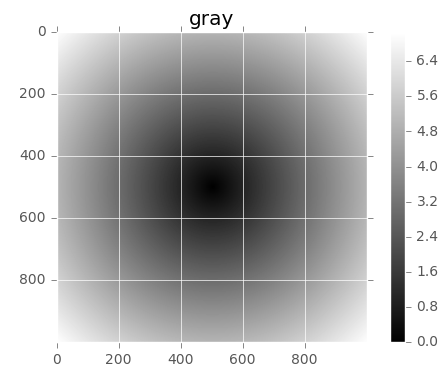
plt.imshow(z,cmap=plt.cm.gray); plt.colorbar()plt.title("gray")
<matplotlib.text.Text at 0x1db84940390>
xarr = np.arange(10)yarr = np.arange(10, 20)cond = np.array([True,False, True,False,False, True,False,False, True, True])
np.where中第二个和第三个参数不用必须是数组。
where在数据分析中一个典型的用法是基于一个数组,产生一个新的数组值。假设我们有一个随机数字生成的矩阵,我们想要把所有的正数变为2,所有的负数变为-2。
用where的话会非常简单:
result = [x if c else y for x,y,c in zip(xarr,yarr,cond)]result
[0, 11, 2, 13, 14, 5, 16, 17, 8, 9]
result = np.where(cond, xarr, yarr)result
array([ 0, 11, 2, 13, 14, 5, 16, 17, 8, 9])
假设我们有一个随机数字生成的矩阵,我们想要把所有的正数变为2,所有的负数变为-2。
用where的话会非常简单
arr = np.random.randn(4,4)arr
array([[-1.7249151 ,  0.47436864,  1.25594568, -0.50147823],
       [ 0.32329558,  0.70147251, -0.84606626, -0.81102393],
       [ 0.56334907, -0.87781646, -1.29420612, -0.882093  ],
       [-2.05570648, -0.60100428, -0.43001513, -0.18520691]])
arr>0
array([[False,  True,  True, False],
       [ True,  True, False, False],
       [ True, False, False, False],
       [False, False, False, False]], dtype=bool)
np.where(arr>0, 2,-2)
array([[-2,  2,  2, -2],
       [ 2,  2, -2, -2],
       [ 2, -2, -2, -2],
       [-2, -2, -2, -2]])
np.where(arr>0, 2, arr)
array([[-1.7249151 ,  2.        ,  2.        , -0.50147823],
       [ 2.        ,  2.        , -0.84606626, -0.81102393],
       [ 2.        , -0.87781646, -1.29420612, -0.882093  ],
       [-2.05570648, -0.60100428, -0.43001513, -0.18520691]])
np.where(arr>0, -2, 2)
array([[ 2, -2, -2,  2],
       [-2, -2,  2,  2],
       [-2,  2,  2,  2],
       [ 2,  2,  2,  2]])
数学和统计方法
一些能计算统计值的数学函数能基于整个数组,或者沿着一个轴,可以使用aggregatios 降维, 比如sum,mean, and std。
下面是一些aggregate statistics (汇总统计)
arr = np.random.randn(5,4)arr
array([[-0.69958443, -2.46355531,  0.19856965,  1.29106598],
       [ 0.46347983,  0.33712368, -1.09018919, -0.21548269],
       [ 0.29535286, -1.39083895, -0.09018223, -0.2594519 ],
       [ 0.90665136, -0.44205849, -0.16239346,  0.31531549],
       [ 0.49731548,  1.08907863, -1.52806488, -0.5010424 ]])
arr.mean()
-0.17244454806253073
np.mean(arr)
-0.17244454806253073
arr.sum()
-3.4488909612506147
arr.mean(axis=1)
array([-0.41837603, -0.12626709, -0.36128006, 0.15437873, -0.11067829])
arr.sum(axis=0)
array([ 1.46321511, -2.87025044, -2.67226011, 0.63040448])
我是过度线--------------------------------------
arr = np.array([0,2,3,4,4,5,66])
arr.cumsum()
array([ 0, 2, 5, 9, 13, 18, 84], dtype=int32)
上面的计算是一个累加的结果,0+2 = 2, 2+3=5...
np.cumsum?
arr = np.array([[23,4,4],[3,5,4,],[42,5,3]])arr
array([[23,  4,  4],
       [ 3,  5,  4],
       [42,  5,  3]])
arr.cumsum(axis=0)
array([[23,  4,  4],
       [26,  9,  8],
       [68, 14, 11]], dtype=int32)
arr.cumsum(axis=1)
array([[23, 27, 31],
       [ 3,  8, 12],
       [42, 47, 50]], dtype=int32)
arr = np.random.randn(100)(arr>0).sum()
55
有其他两个办法,any和all, 对于布尔数组特别有用,any 检测数组中只要有一个Ture就返回,就是Ture, 而all,检测数组中所有都是True,才返回True
bools = np.array([False, False, True, True])
bools.any()
True
bools.all()
False
Sorting(排序)
np.random.randn?
arr = np.random.randn(6)arr
array([ 0.3934821 ,  0.95045695,  0.08114809,  0.71009844, -0.58873837,
       -0.39691479])
arr
array([ 0.3934821 ,  0.95045695,  0.08114809,  0.71009844, -0.58873837,
       -0.39691479])
arr.sort()arr
array([-0.58873837, -0.39691479,  0.08114809,  0.3934821 ,  0.71009844,
        0.95045695])
arr = np.random.randn(5,3)arr
array([[ 2.09807311,  0.76233307,  0.50202059],
       [-1.72025055, -0.16630714, -1.47464429],
       [ 2.82788532, -1.25434574,  0.97145056],
       [ 0.58417455,  0.51401424, -0.4251397 ],
       [ 0.89538709,  1.15031466, -0.66813715]])
arr.sort()arr
array([[ 0.50202059,  0.76233307,  2.09807311],
       [-1.72025055, -1.47464429, -0.16630714],
       [-1.25434574,  0.97145056,  2.82788532],
       [-0.4251397 ,  0.51401424,  0.58417455],
       [-0.66813715,  0.89538709,  1.15031466]])
arr.sort(0)arr
array([[-1.72025055, -1.47464429, -0.16630714],
       [-1.25434574,  0.51401424,  0.58417455],
       [-0.66813715,  0.76233307,  1.15031466],
       [-0.4251397 ,  0.89538709,  2.09807311],
       [ 0.50202059,  0.97145056,  2.82788532]])
