@JeemyJohn
2018-01-23T04:18:32.000000Z
字数 9667
阅读 1673
LightGBM大战XGBoost,谁将夺得桂冠?
机器学习
0.引言
如果你是一个机器学习社区的活跃成员,你一定知道 提升机器(Boosting Machine)以及它们的能力。提升机器从AdaBoost发展到目前最流行的XGBoost。XGBoost实际上已经成为赢得在Kaggle比赛中公认的算法。这很简单,因为他极其强大。但是,如果数据量极其的大,XGBoost也需要花费很长的时间去训练。
绝大多数人可能对 Light Gradient Boosting 不熟悉,但是读完本文后你就会对他们很熟悉。一个很自然的问题将进入你的思索:为什么又会出现另一个提升机器算法?它比XGBoost要好吗?
注意:本文假设读者已经对 GBMs 和 XGBoost 算法有一定的了解。如果你不了解他们,请先了解一下他们的原理再来学习本文。
1. 什么是LightGBM
LightGBM是个快速的、分布式的、高性能的基于决策树算法的梯度提升框架。可用于排序、分类、回归以及很多其他的机器学习任务中。
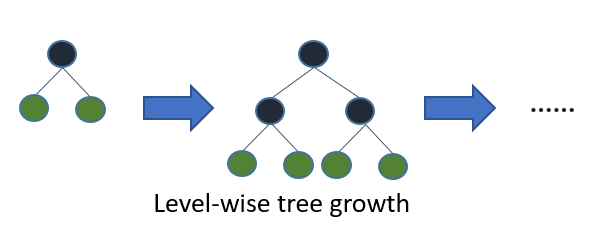
因为他是基于决策树算法的,它采用最优的leaf-wise策略分裂叶子节点,然而其它的提升算法分裂树一般采用的是depth-wise或者level-wise而不是leaf-wise。因此,在LightGBM算法中,当增长到相同的叶子节点,leaf-wise算法比level-wise算法减少更多的loss。因此导致更高的精度,而其他的任何已存在的提升算法都不能够达。与此同时,它的速度也让人感到震惊,这就是该算法名字 Light 的原因。
前文是一个由LightGBM算法作者的概要式的描述来简要地解释LightGBM的不同之处。
- XGBoost中决策树的增长方式示意图
- LightGBM中决策树的增长方式示意图
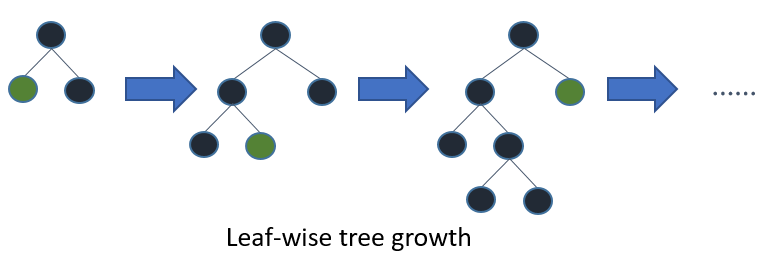
Leaf-Wise分裂导致复杂性的增加并且可能导致过拟合。但是这是可以通过设置另一个参数 max-depth 来克服,它分裂产生的树的最大深度。
接下来我们将介绍安装LightGBM的步骤使用它来跑一个模型。我们将对比LightGBM和XGBoost的实验结果来证明你应该使用LightGBM在一种轻轻的方式(Light Manner)。
2. LightGBM的优势
首先让我们看一看LightGBM的优势。
更快的训练速度和更高的效率: LightGBM使用基于直方图的算法。例如,它将连续的特征值分桶(buckets)装进离散的箱子(bins),这是的训练过程中变得更快。
更低的内存占用:使用离散的箱子(bins)保存并替换连续值导致更少的内存占用。
更高的准确率(相比于其他任何提升算法) : 它通过leaf-wise分裂方法产生比level-wise分裂方法更复杂的树,这就是实现更高准确率的主要因素。然而,它有时候或导致过拟合,但是我们可以通过设置 max-depth 参数来防止过拟合的发生。
大数据处理能力: 相比于XGBoost,由于它在训练时间上的缩减,它同样能够具有处理大数据的能力。
支持并行学习
3. 安装LightGBM
本节介绍如何在各种操作系统下安装LightGBM。众所周知,桌面系统目前使用最多的就是Windows、Linux和macOS,因此,就依次介绍如何在这三种操作系统下安装LightGBM。
3.1 Windows
对于Windows操作系统,由于其并非开源操作系统,因此一直以来Windows系统对开发者来说并不友好。我们需要安装相应的编译环境才能对LightGBM源代码进行编译。对于Windows下的底层C/C++编译环境,目前主要有微软自己的Visual Studio(或者MSBuild)或者开源的MinGW64,下面我们依次介绍这两种编译环境下的LightGBM的安装。
注意,对于以下两种编译环境,我们都共同需要确保系统已经安装Windows下的Git和CMake工具。
- 3.1.1 基于Visual Studio(MSBuild)环境
git clone --recursive https://github.com/Microsoft/LightGBMcd LightGBMmkdir buildcd buildcmake -DCMAKE_GENERATOR_PLATFORM=x64 ..cmake --build . --target ALL_BUILD --config Release
最终编译生成的exe和dll会在 LightGBM/Release 目录下。
- 3.1.2 基于MinGW64环境
git clone --recursive https://github.com/Microsoft/LightGBMcd LightGBMmkdir buildcd buildcmake -G "MinGW Makefiles" ..mingw32-make.exe -j
最终编译生成的exe和dll会在 LightGBM/ 目录下。
3.2 Linux
在Linux系统下,我们同样适用cmake进行编译,运行如下的shell命令:
git clone --recursive https://github.com/Microsoft/LightGBMcd LightGBMmkdir buildcd buildcmake ..make -j
3.3 macOS
LightGBM依赖OpenMP来编译,但是它不支持苹果的Clang,请使用gcc/g++替代。运行如下的命令进行编译:
brew install cmakebrew install gcc --without-multilibgit clone --recursive https://github.com/Microsoft/LightGBMcd LightGBMmkdir buildcd buildcmake ..make -j
现在,在我们投入研究构建我们第一个LightGBM模型之前,让我们看一下LightGBM的一些参数,以更好的了解其基本过程。
4. LightGBM的重要参数
task: 默认值=train,可选项=train,prediction;指定我们希望执行的任务,该任务有两种类型:训练 和 预测;
application: 默认值=regression,type=enum,options=options;
- regression: 执行回归任务;
- binary:二分类;
- multiclass:多分类;
- lambdarank:lambrank应用;
data: type=string;training data,LightGBM将从这些数据中进行训练;
num_iterations: 默认值为100,类型为int。表示提升迭代次数,也就是提升树的棵树;
num_leaves: 每个树上的叶子数,默认值为31,类型为int;
device: 默认值=cpu;可选项:cpu,gpu。也就是我们使用什么类型的设备去训练我们的模型。选择GPU会使得训练过程更快;
min_data_in_leaf: 每个叶子上的最少数据;
feature_fraction: 默认值为1;指定每次迭代所需要的特征部分;
bagging_fraction: 默认值为1;指定每次迭代所需要的数据部分,并且它通常是被用来提升训练速度和避免过拟合的。
min_gain_to_split: 默认值为1;执行分裂的最小的信息增益;
max_bin: 最大的桶的数量,用来装数值的;
min_data_in_bin: 每个桶内最少的数据量;
num_threads: 默认值为OpenMP_default,类型为int。指定LightGBM算法运行时线程的数量;
label: 类型为string;指定标签列;
categorical_feature: 类型为string;指定我们想要进行模型训练所使用的特征类别;
num_class: 默认值为1,类型为int;仅仅需要在多分类的场合。
5. LightGBM与XGBoost对比
现在让我们通过在同一个数据集上进行训练,对比一下LightGBM和XGBoost的性能差异。
在这里我们使用的数据集来自很多国家的个人信息。我们的目标是基于其他的基本信息来预测每个人的年收入是否超过50K(<=50K 和 >50K两种)。该数据集包含32561个被观测者和14个描述每个个体的特征。这里是数据集的链接: http://archive.ics.uci.edu/ml/datasets/Adult。
通过对数据集的预测变量有一个正确的理解这样你才能够更好的理解下面的代码。
#importing standard librariesimport numpy as npimport pandas as pdfrom pandas import Series, DataFrame#import lightgbm and xgboostimport lightgbm as lgbimport xgboost as xgb#loading our training dataset 'adult.csv' with name 'data' using pandasdata=pd.read_csv('adult.csv',header=None)#Assigning names to the columnsdata.columns=['age','workclass','fnlwgt','education','education-num','marital_Status','occupation','relationship','race','sex','capital_gain','capital_loss','hours_per_week','native_country','Income']#glimpse of the datasetdata.head()# Label Encoding our target variablefrom sklearn.preprocessing import LabelEncoder,OneHotEncoderl=LabelEncoder()l.fit(data.Income)l.classes_data.Income=Series(l.transform(data.Income)) #label encoding our target variabledata.Income.value_counts()#One Hot Encoding of the Categorical featuresone_hot_workclass=pd.get_dummies(data.workclass)one_hot_education=pd.get_dummies(data.education)one_hot_marital_Status=pd.get_dummies(data.marital_Status)one_hot_occupation=pd.get_dummies(data.occupation)one_hot_relationship=pd.get_dummies(data.relationship)one_hot_race=pd.get_dummies(data.race)one_hot_sex=pd.get_dummies(data.sex)one_hot_native_country=pd.get_dummies(data.native_country)#removing categorical featuresdata.drop(['workclass','education','marital_Status','occupation','relationship','race','sex','native_country'],axis=1,inplace=True)#Merging one hot encoded features with our dataset 'data'data=pd.concat([data,one_hot_workclass,one_hot_education,one_hot_marital_Status,one_hot_occupation,one_hot_relationship,one_hot_race,one_hot_sex,one_hot_native_country],axis=1)#removing dulpicate columns_, i = np.unique(data.columns, return_index=True)data=data.iloc[:, i]#Here our target variable is 'Income' with values as 1 or 0.#Separating our data into features dataset x and our target dataset yx=data.drop('Income',axis=1)y=data.Income#Imputing missing values in our target variabley.fillna(y.mode()[0],inplace=True)#Now splitting our dataset into test and trainfrom sklearn.model_selection import train_test_splitx_train,x_test,y_train,y_test=train_test_split(x,y,test_size=.3)
5.1 使用XGBoost
#The data is stored in a DMatrix object#label is used to define our outcome variabledtrain=xgb.DMatrix(x_train,label=y_train)dtest=xgb.DMatrix(x_test)#setting parameters for xgboostparameters={'max_depth':7, 'eta':1, 'silent':1,'objective':'binary:logistic','eval_metric':'auc','learning_rate':.05}#training our modelnum_round=50from datetime import datetimestart = datetime.now()xg=xgb.train(parameters,dtrain,num_round)stop = datetime.now()#Execution time of the modelexecution_time_xgb = stop-startprint(execution_time_xgb)#datetime.timedelta( , , ) representation => (days , seconds , microseconds)#now predicting our model on test setypred=xg.predict(dtest)print(ypred)#Converting probabilities into 1 or 0for i in range(0,9769):if ypred[i]>=.5: # setting threshold to .5ypred[i]=1else:ypred[i]=0#calculating accuracy of our modelfrom sklearn.metrics import accuracy_scoreaccuracy_xgb = accuracy_score(y_test,ypred)print(accuracy_xgb)
5.2 使用LightGBM
train_data=lgb.Dataset(x_train,label=y_train)setting parameters for lightgbmparam = {'num_leaves':150, 'objective':'binary','max_depth':7,'learning_rate':.05,'max_bin':200}param['metric'] = ['auc', 'binary_logloss']#Here we have set max_depth in xgb and LightGBM to 7 to have a fair comparison between the two.#training our model using light gbmnum_round=50start=datetime.now()lgbm=lgb.train(param,train_data,num_round)stop=datetime.now()#Execution time of the modelexecution_time_lgbm = stop-startprint(execution_time_lgbm)#predicting on test setypred2=lgbm.predict(x_test)print(ypred2[0:5]) # showing first 5 predictions#converting probabilities into 0 or 1for i in range(0,9769):if ypred2[i]>=.5: # setting threshold to .5ypred2[i]=1else:ypred2[i]=0#calculating accuracyaccuracy_lgbm = accuracy_score(ypred2,y_test)accuracy_lgbmy_test.value_counts()from sklearn.metrics import roc_auc_score#calculating roc_auc_score for xgboostauc_xgb = roc_auc_score(y_test,ypred)print(auc_xgb)#calculating roc_auc_score for light gbm.auc_lgbm = roc_auc_score(y_test,ypred2)auc_lgbm comparison_dict = {'accuracy score':(accuracy_lgbm,accuracy_xgb),'auc score':(auc_lgbm,auc_xgb),'execution time':(execution_time_lgbm,execution_time_xgb)}#Creating a dataframe ‘comparison_df’ for comparing the performance of Lightgbm and xgb.comparison_df = DataFrame(comparison_dict)comparison_df.index= ['LightGBM','xgboost']print(comparison_df)
5.3 性能对比
下面的表格列出了算法的各项指标对比结果:
| 算法 | accuracy score | auc score | 执行时间(S) |
|---|---|---|---|
| LightGBM | 0.861501 | 0.764492 | 0.283759 |
| XGBoost | 0.861398 | 0.764284 | 2.047220 |
从上述的性能对比结果来看,LightGBM对比XGBoost的准确率和AUC值都只有很小的提升。但是,一个至关重要的差别是模型训练过程的执行时间。LightGBM的训练速度几乎比XGBoost快7倍,并且随着训练数据量的增大差别会越来越明显。
这证明了LightGBM在大数据集上训练的巨大的优势,尤其是在具有时间限制的对比中。
5.4 详细对比
| 对比项 | XGBoost | LightGBM |
|---|---|---|
| 正则化 | L1/L2 | L1/L2 |
| 列采样 | yes | yes |
| Exact Gradient | yes | yes |
| 近似算法 | yes | no |
| 稀疏数据 | yes | yes |
| 分布式并行 | yes | yes |
| 缓存 | yes | no |
| out of core | yes | no |
| 加权数据 | yes | yes |
| 树增长方式 | level-wise | leaf-wise |
| 基于算法 | pre-sorted | histgram |
| 最大树深度控制 | 无 | 有 |
| dropout | no | yes |
| Bagging | yes | yes |
| 用途 | 回归、分类、rank | 回归、分类、lambdrank |
| GPU支持 | no | yes |
| 网络通信 | point-to-point | collective-communication |
| CategoricalFeatures | 无优化 | 优化 |
| Continued train with input GBDT model | no | yes |
| Continued train with input | no | yes |
| Early Stopping(both training and prediction) | no | yes |
6. LightGBM的参数调优
LightGBM使用基于depth-wise的分裂的leaf-wise分裂算法,这使得它能够更快地收敛。但是,它也会导致过拟合。因此,这里给出一个LightGBM参数调优的快速指南。
6.1 为了最好的拟合
num_leaves:这个参数是用来设置组成每棵树的叶子的数量。num_leaves 和 max_depth理论上的联系是: num_leaves = 2^(max_depth)。然而,但是如果使用LightGBM的情况下,这种估计就不正确了:因为它使用了leaf_wise而不是depth_wise分裂叶子节点。因此,num_leaves必须设置为一个小于2^(max_depth)的值。否则,他将可能会导致过拟合。LightGBM的num_leave和max_depth这两个参数之间没有直接的联系。因此,我们一定不要把两者联系在一起。
min_data_in_leaf : 它也是一个用来解决过拟合的非常重要的参数。把它的值设置的特别小可能会导致过拟合,因此,我们需要对其进行相应的设置。因此,对于大数据集来说,我们应该把它的值设置为几百到几千。
max_depth: 它指定了每棵树的最大深度或者它能够生长的层数上限。
6.2 为了更快的速度
bagging_fraction : 它被用来执行更快的结果装袋;
feature_fraction : 设置每一次迭代所使用的特征子集;
max_bin : max_bin的值越小越能够节省更多的时间:当它将特征值分桶装进不同的桶中的时候,这在计算上是很便宜的。
6.3 为了更高的准确率
使用更大的训练数据集;
num_leaves : 把它设置得过大会使得树的深度更高、准确率也随之提升,但是这会导致过拟合。因此它的值被设置地过高不好。
max_bin : 该值设置地越高导致的效果和num_leaves的增长效果是相似的,并且会导致我们的训练过程变得缓慢。
7. 结束语
在本文中,我给出了关于LightGBM的直观的想法。现在使用该算法的一个缺点是它的用户基础太少了。但是种局面将很快得到改变。该算法除了比XGBoost更精确和节省时间以外,现在被使用的很少的原因是他的可用文档太少。
然而,该算法已经展现出在结果上远超其他已存在的提升算法。我强烈推荐你去使用LightGBM与其他的提升算法,并且自己亲自感受一下他们之间的不同。
也许现在说LightGBM算法称雄还为时过早。但是,他确实挑战了XGBoost的地位。给你一句警告:就像其他任何机器学习算法一样,在使用它进行模型训练之前确保你正确的调试了参数。

