Planet: Understanding the Amazon from Space

机器学习

---

East China Normal University

10152510119 Ziqi Xu,
10152510217 Weiwen Chen,
10152510208 Jiale Lin,
10142130229 Ming Zhong.

1 Abstract

1.1 Background

Deforestation is one of the most serious environmental problems in recent years. Every minute, the world loses an area of forest the size of 48 football fields and deforestation in the Amazon Basin accounts for the largest share. Moreover, due to Amazon Basin.s significant impact on biodiversity and global climate. Deforestation in Amazon Basin has contributed to different devastating effects. Better data about the location of deforestation and human encroachment on forests can help various group of people respond more quickly and effectively.

1.2 Motivation

With images collected by satellites, we are able to track changes in forest and differentiate between different causes of forest loss. We challenge ourselves to label satellite image chips with atmospheric conditions and various classes of land use. With convolutional neural network and other machine learning algorithms, we apply different methods to learn about the patterns of different kinds of land use from a large amount of labeled images and solve the classification problem of new pictures. Resulting algorithms will help people know about the condition of deforestation and try to solve the problem of deforestation.

2 Preliminary

2.1 Data Process

We download data from a contest on kaggle1, According to the official provided pictures, these pictures are all 256 ∗ 256 pixels. And there are 17 tags of these pictures including 4 kinds of weather, 7 kinds of ordinary landform and 6 kinds of rare landform. Here is 17 tags:

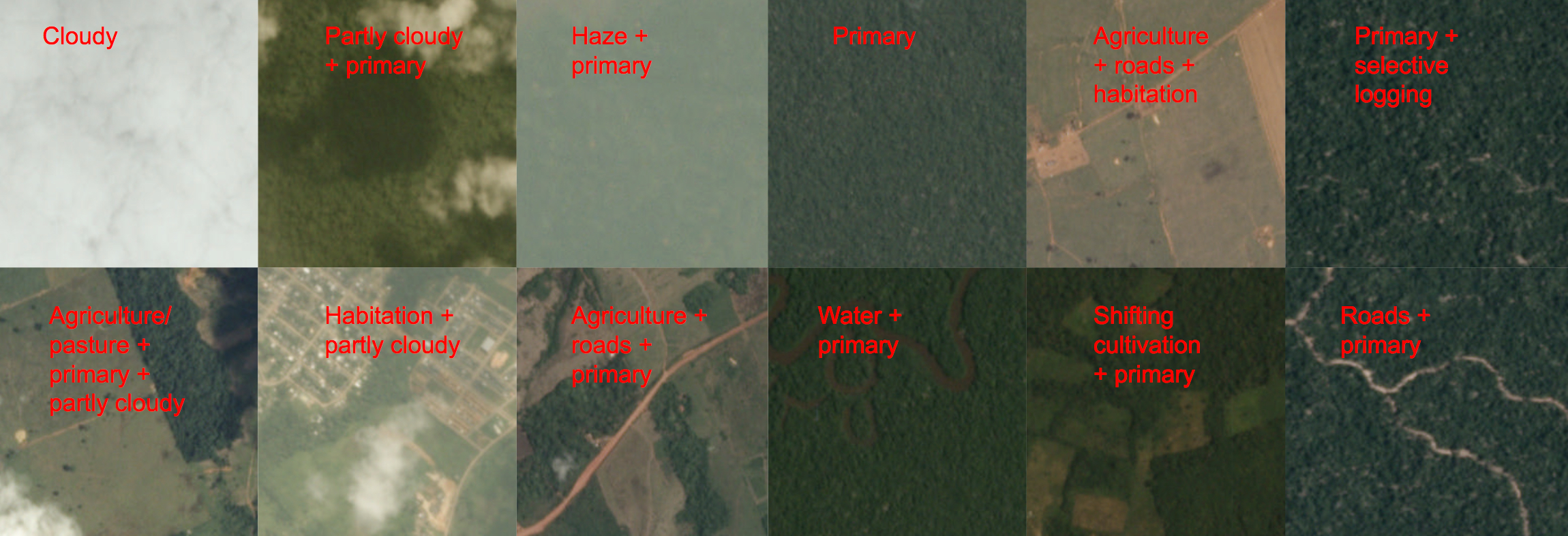
Weather: Clear, Partly Cloudy, Cloudy, Haze.
Especially, if there is Cloudy, there will not be any other weather tags.
Ordinary Landform: Primary Rain Forest, Water (Rivers & Lakes), Habitation, Agriculture, Road, Cultivation, Bare Ground.
Rare Landform: Slash and Burn, Selective Logging, Blooming, Conventional Mining, ”Artisinal” MiningßBlow Down.

So from the preliminary data analysis, we can figure out that this is a Multi-Label problem. To solve a multi-label problem, we have two solutions. First, we can split the problem to several binary classification problems. The advantage of this solution is that this model may cost fewer time, but this model has a fatal disadvantage that this model ignore the connection between each tags. Second, we can use a model to train these 17 tags together. The advantage of this solution is that it contain the potential connection between each tags, but the biggest problems are the Memory and Process speed.

2.2 Evaluation

According to the Kaggle Overview, we use the F2-score to examine our models, here is the def- inition of F2-score:

$$(1+\beta^2)\frac{pr}{\beta^2 p+r} where p = \frac{tp}{tp+fp}, r = \frac{tp}{tp+fn}, \beta=2$$
here p is the precision, r is the recall.

3 Design Challenges

With more than 40000 images in the training data, it necessary and urgent to design an algorithm that has high accuracy of prediction and relatively short training time because training convolutional neural network is an extremely time-consuming and storage-consuming task. Furthermore, due to the limit of the resolution of satellite images and the limit of shoot environment at an extremely high altitude, the satellite images are not clear enough and the images all appear to have some haze over the actual landscape and artificial land sites. All these flaw of the given data add to the difficulty of the classification of these images. Last but not least, the partial similarity between features of different kinds of land use is one of the most critical and complicated difficulties to be solved when we need to find the pattern of a specific kind of land use.

4 Architecture of Algorithm Models

With the intention to solve the problems above, we have built two different model to get an efficient and highly usable solution. This part of the report will present a detailed introduction of the architecture of the algorithms we used and the techniques we have applied.

4.1 Model 1–Based on Tensorflow

The first model is a relatively simple model constructed using tensorflow version 1.1 on python 3.5.2. In this model, we perform the k-fold validation on the dataset. K is determined by the value of the variable named nfolds. The whole dataset is randomly split into training data and validation data. Afterwards, we use a sequential model for training. In the neural network, there are three layers in total. The first two layers consist of a convolutional layer and a maxpooling layer and, every time of iteration, a variable named kp adjusts the rate of the neurons chosen randomly and set to zero. The first layer consists of two convolutional layers and a maxpooling layer. The size of the 16 filters in the convolutional layers is 3*3*3 and the maxpooling size is 2*2. In the second layer, the size of the 32 filters in the convolutional layers becomes 3*3*16 and all other parameters remain the same. Finally, the fourth layer is a fully connected layer. The drop-out rate in this layer is also determined by the value of the variable kp, which is generally set at 0.4.

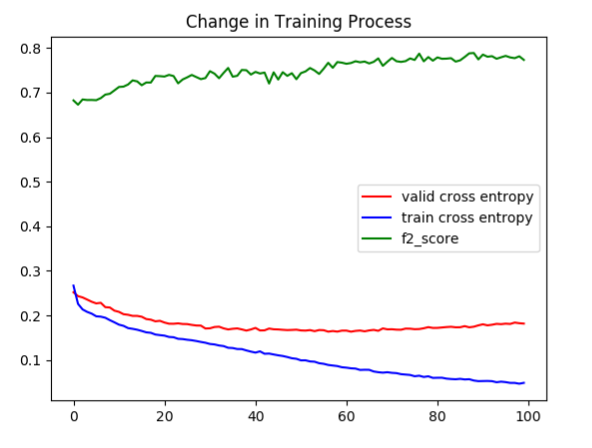
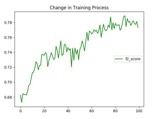
As elaborated in the following visualizations, we can find that the training cross entropy goes down to about 0.05 while the average validation accuracy stops at about 0.16 and even shows a tendency of slight increasing. The conclusion we can make from the plots is that the model trained may be overfitting, which is a problem settled in the second model. The probable method to deal with the overfitting include the regularization, drop out, training sample augmentation. We implement the first two methods and give up the attempt of the third method due to the memory limit. However, the regularization doesn.t matter (the code is in the note part of cnn.py). The final result this model achieve, measured in f2 score is 0.79.

4.2 Model 2–Based on Keras

Due to the preliminary data process, we find that this is a multi-label problem.

The second model is implemented using tensorflow-gpu version 1.4, keras and other packages such as sklearn. It is a bit more complicated than the first model but it also has better performance. In this model, we perform the k-fold validation on the dataset. K is determined by the value of the variable named nfolds. The dataset is randomly split into training data and validation data. After- wards, we use a sequential model for training. In the neural network, there are four layers in total. Three of the four layers consist of two convolutional layers and a maxpooling layer and, every time of iteration, 25% of the neurons in these layers are chosen randomly and set to zero. The kernel size of the first layer is 32, and we have two convolutional layers in this layer. The difference between these two layers is that the first convolutional layer calculates border data, so the shape of input and output will be identical. The fourth layer is a fully connected layer and the random drop-out rate is 50%. In the training process, the learning rate decreases as after completing the training of certain number of epochs from 0.001 to 0.0001 and then to 0.00001.

To give a more detailed explanation about this model, the report will go through the detail of implementation of every layer. The first layer consists of two convolutional layers and a maxpooling layer. The size of the 32 filters in the convolutional layers is 3*3*3 and the maxpooling size is 2*2. In the second layer, the size of the 64 filters in the convolutional layers becomes 3*3*32 and all the other remain the same. In the third layer, the size of the 128 filters in the convolutional layers becomes 3*3*64. Finally, in the fourth layer, there is a dense layer using ReLU as activation function and a dense layer using sigmoid function as activation function.

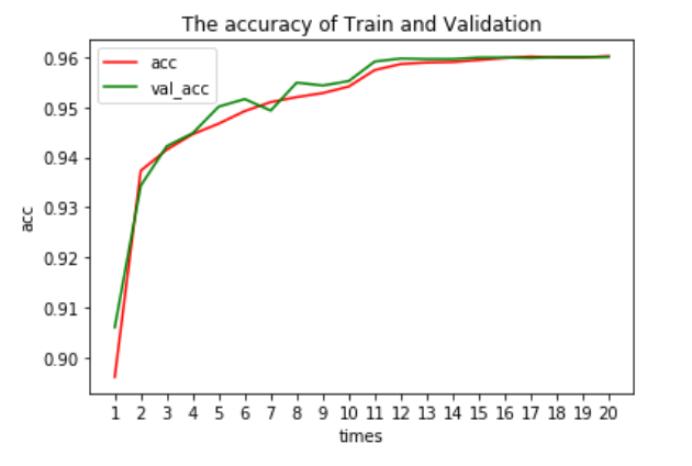
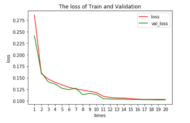
As elaborated in the following visualizations, at the beginning, the accuracy of training and vali- dation sets of our model 2 is about 0.89 and 0.90. It’s quite good. And the binary crossentropy loss of training and validation sets of our model 2 is about 0.28 and 0.24. After training process, the accuracy of both sets finally levels out at 0.96. And the binary crossentropy loss of both sets finally levels out at 0.10.

So according to the data, we can draw a conclusion that our model do not get overfitting and underfitting. We have a good model.

Here is part of our code of Model 2:

model = Sequential ()
model.add(BatchNormalization(input shape=(64, 64,3)))
model.add(Conv2D(32, kernel size=(3, 3),padding=’same’, activation=’relu’)) 
model.add(Conv2D(32, (3, 3), activation=’relu’))
model.add(MaxPooling2D(pool size=(2, 2))) 
model.add(Dropout(0.25))
model.add(Conv2D(64, kernel size=(3, 3),padding=’same’, activation=’relu’)) 
model.add(Conv2D(64, (3, 3), activation=’relu’))
model.add(MaxPooling2D(pool size=(2, 2)))
model.add(Dropout(0.25))
model.add(Conv2D(128, kernel size=(3, 3),padding=’same’, activation=’relu’)) 
model.add(Conv2D(128, (3, 3), activation=’relu’))
model.add(MaxPooling2D(pool size=(2, 2)))
model.add(Dropout(0.25))
model.add(Flatten())
model.add(Dense(256, activation=’relu ’))
model.add(BatchNormalization()) 
model.add(Dropout(0.5))
model.add(Dense(17, activation=’sigmoid’))
epochs arr = [20, 5, 5]
learn rates = [0.001, 0.0001, 0.00001]
for learn rate , epochs in zip(learn rates , epochs arr):
    opt = optimizers .Adam( lr=learn   rate )
    model.compile(loss=’binary crossentropy’,optimizer=opt,metrics=[’accuracy’])
    callbacks = [EarlyStopping(monitor=’val loss’, patience=2, verbose=0), ModelCheckpoint(kfold weights path , monitor=’val loss’, save best only=True, verbose=0)]
    model.fit(x = X train, y= Y train, validation data=(X valid, Y valid),batch size=128,verbose=2, epochs=epochs , callbacks=callbacks , shuffle=True)

5 Innovative Aspects

When we apply the first model to solve the classification problem, due to the memory limit, the samples we used only include the first 10000 pictures. (However, when it comes to the second model, we use the whole 40000 pictures since the computer.s memory is larger). The pictures used are resized to the form 64*64*3. Apart from every layer introduced above, we use the sigmoid cross entropy as the loss function. In addition, the learning rate set is 0.001 and the optimizer using is Adam optimizer. We divide the training sample into 5 parts and do the cross validation. The fourth layer is directly connected to the 17 labels, which are represented by a 1*17 vector with 1 denoting the existence of the label and 0 denoting the opposite. We train the model with the batch size 100 and use 100 iterations to fit the whole 8000 pictures.

6 Unsolved Problems

We tried to use some distributed computing systems to accelerate the training process. The first service that we considered to use were the GPU service or the machine learning platform offered by AWS. Nevertheless, unfortunately, we were not allowed to buy the AWS services without a registered company license in China. So we tried to use service offered by a Chinese company called AliCloud but the price was very high and this company forces its client to keep the service running for 24 hours a day otherwise they will delete your data so we couldn.t afford that. Besides, the machine learning services offered by AliCloud was still a demo so it was not actually usable for our project. Because of those reasons mentioned above, we were not able to deploy our model on distributed computing systems and we just kept running our model with our personal computers.

7 Submission

What’s more, we also use the model 2–based on Keras to test the test-jpg and we have a submis- sion file. Then we upload the file to Kaggle. Here is the result:

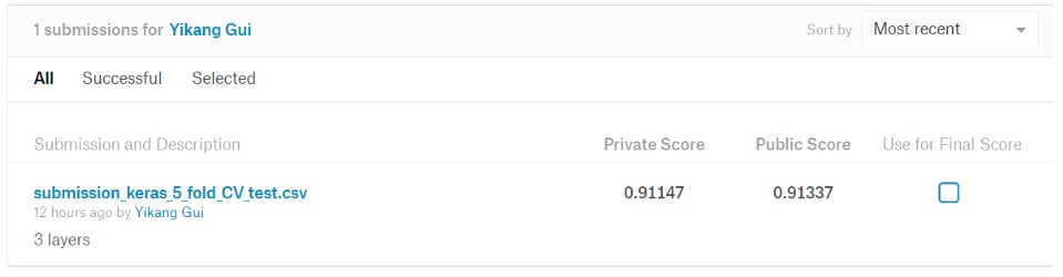
As you can see, the final result of model 2 achieve, measured in f2 score, is 0.91337.

8 Suggestion

1. Because our GPU memory is limited to 4GB and our tensorflow is based on GPU, we cannot augment the raw picture data, like rotation, Random Crop, Horizontal/Vertiacal Flip. So our further plan is to run our model on Cloud Server with larger GPU memory.
2. Our model 1&2 are both designed with CNN, and we’d like to try other algorithm, like RNN, Random Forests, Adaboost.

9. Reference

1. Planet: Understanding the Amazon from Space, https://www.kaggle.com/c/planet-understanding-the-amazon-from-space

2. Single Image Haze Removal Using Dark Channel Prior, http://blog.csdn.net/songhhll/article/details/12612681