The Effects of Climate Change on Instability of Countries

未分类

---

Abstract: Climate change has an influence on the fragility of a country, so it’s extremely significant to anticipate possible impacts. Our goal is to build a model to better classify the category of countries based on their fragility. This model can give an optimal explanation of a country’s fragility, and an accurate prediction of the foreseeable changing of a country’s fragility. What’s more, we find out that our model can perform well in mitigating the risk of climate change.
To illustrate our model more clearly, we start with the discussion of how to choose the indicators. We choose nine indicators which related to the climate change closely, including Proved Water, CO2 emissions, Land Use, Forest Area, etc. The model of how climate change affects the fragility is based on these nine indicators. In addition, combined the K-means algorithm and the Mean Lift algorithm, we complete our clustering analysis. Therefore, in our model, the category of countries is classified into three types: fragile countries, vulnerable countries and stable countries.
In our Logistic Regression Model, we take three clustering centers into consideration. Using Clementine12.0 (software), we find out the logistic regression function and three feature indicators: Proved Water, CO2 emissions and Land Use. Besides, the correlation coefficients are provided, so we can identify how climate change increases the fragility of a country. In our C&R Trees Model, we selected three feature indicators by comparing the “Variable Importance” of different indicators. Then, we make a prediction of a country’s fragility based on the analysis of the training set and the testing set. Although we can’t obtain the complete data of all countries in 2017, our model predictions are still accurate enough. Furthermore, comparing the specific proportion we calculate in our model and the given threshold, we can easily determine the state of a country’s interventions and find out whether the risk of climate change is mitigated. In addition, we make further consideration and improvement for applying our model in a smaller or larger range.

Keywords: Cluster, Regression, Decision-making Tree, Random Forest, Climate Change, fragility

---

1 Introduction

1.1 Background

Today and every day, the trend of global warming is gradually increasing. It seems that weather conditions are changing gradually so far and will be similar in the predictable future, but researchers suggest that adverse climate condition would develop much more abruptly once the temperature rises above some threshold. Such an abrupt climate change could result in harsher winter weather conditions, food shortages, decreased availability and quality of fresh water, and interrupted energy supplies in regions all over the world. These resource constraints could lead to global and local carrying capacities reduction. Frequent skirmishes, battles, and even wars would happen due to rising living pressure and relatively worse living condition. Without powerful government, this climate change and its follow-on effects could become a challenge to a country. Facing this challenge, it's significant to create an improved, reasonable model which could be used to investigate a wider range of scenarios and predict how will the climate change influence the stability of a country. And it's of vital importance for us to create a fragility model to anticipate which countries are most vulnerable and fragile to abrupt climate change.

1.2 Literature Review

Correlations between different indicators

The fragility of a country is related to various of indicators which are inter-related. We should not only consider the scores in 12 indicators, but also other climate change indicators.

Common problems of selecting relative data:

1. The data of various of countries in different years is incomplete, which extremely limits our modelling process.
2. The selection of new indicators is subjective, leading different model results.
3. Different clustering algorithms all have its own advantages and limitations, so the selection and combination process is flexible.
4. The method of filling the missing value has a possible influence on the result of the model.

The methods and rules of dealing with outliers:

1. Directly retain the outliers for subsequent data processing.
2. Modify the outliers and retain them for subsequent data processing.
3. Eliminate outliers without additional observation values.
4. Eliminate outliers and adding new observation values or replacing them with appropriate interpolation values.

Since the indicators in different countries are affected by many special factors, we choose to retain them and get our final model.

1.3 Restatement of the Problem

We are required to design a model to determine a country's fragility and simultaneously measure the impact of climate change. Then we are expected to explain how climate change may have affected the fragility of a specific country. Improvement of the efficiency, accuracy, and stability of our model is also considered. In addition, we also need to determine which state driven interventions could mitigate the risk of climate change and prevent a country from being fragile. Besides, it's of vital significance to anticipate the total cost of the effective intervention. Finally, indispensable change needs to be made as we shrink and expand the range of scenarios in our model.

2 Data Introduction

2.1 Selection of Indicators

(1)What is Climate Change?

Climate Capacity, as a new concept, works as a measurement for adapting to climate change. The Climate Capacity appears to depend largely on factors such as climatic resources carrying capability, water resources carrying capability, ecological carrying capability, land carrying capability and environmental capability. So, we choose these indicators to measure the influences of climate change.

Climate Change has six levels of details:

Temperature Change

It is a key element which would make a great influence on sea-level rise, leading the reluctant movement of coastal residents. The cold weather and the drought will reduce the happiness of living and cause food shortages and so on.

Land Use

To measure the influence of land use in different years more clearly, land use total, land cover and the percent of land use are included in the modelling process.

Population

We consider the population in two ways: the total annual population which represents the developments of a country and the population density which represents the living pressure of a country.

Water sources

Proved water resource satisfies the development of a country because it ensures the quality of the residents' daily lives.

$CO_2$ emissions

This indicator works as a connection between the sea-level rising, temperature changing, population and so on.

Forest area

Since the forests are related to the $CO_2$ emissions, we have to evaluate the fragility of a country on the dimension of protecting forest areas.

(2)Addition

Although the fragility of a country depends on the climate change in our assumption, the Government Expenditure works as a tool to reduce the influence of climate change and keep the country as stable as possible. We add a new indicator as Government Expenditure, depending on whether the government officers are willing to keep the country stable and the economic strength.
Finally, we collect all data from the database of FAO and the World Bank.

Table[2-1]

Symbols used

Symbol	Unit	Definition
C1	score	Security Apparatus
C2	score	Factionalized Elites
C3	score	Group Grievance
E1	score	Economy
E2	score	Economic Inequality
E3	score	Human Flight and Brain Drain
P1	score	State Legitimacy
P2	score	Public Services
P3	score	Human Rights
S1	score	Demographic Pressures
S2	score	Refugees and IDPs
X1	score	External Intervention
ET	Degrees Celsius	Temperature change every year
GL	Gigagrams	Land Use Total
OA	1000 persons	Annual population
GV	Ha/ Gigagrams	Cultivation of Organic Soils
LC	1000 ha	Land Cover
FA	%	Forest area (% of land area)
WS	% of population with access	Improved water source
$CO_2$	metric tons per capita	$CO_2$ emissions
PD	per kilometer of land area	Population density
GE	millions	Government Expenditure

2.2 Data Processing Introduction

Dividing the samples according to the ratio of 2:1, we construct our model with 2/3 of the dataset as the training set and 1/3 of the dataset as the testing set.

2.3 Descriptive Statistical Analysis

In this section, we mainly make a descriptive statistical analysis of the variables used above. Statistical analysis was performed on the categorical variables and numerical variables.

Table[2-3]
Descriptive statistical analysis of the indicators

Indicators	Minimum	Maximum	Mean	Standard Deviation	Variance
ForestArea	.000	98.306	31.21422	23.551335	554.665
$CO_2$ emissions	.044	45.423	4.66645	6.214168	38.616
PopulationDensity	1.882	7714.702	190.17737	613.177172	375986.244
ProvedWater	40.000	100.000	88.33041	14.500384	210.261
GovernmentSpending	103	1780850000	18631265	136802555	18714939090702944
LandCover	.027	1984.852	178.90717	362.622339	131494.961
Land	.120	98.400	38.00114	25.370147	643.644
Cropland organic soils	.000	3910355.000	81646.82784	333992.757160	111551161835.329
Temperature change	.000	2.623	1.12834	.562862	.317

3 Clustering Analysis Model

Cluster analysis, as the basic composition of data analysis, plays a significant role in our modelling. On one hand, many tools and algorithms for cluster analysis have been created based on different principles, such as the distance or similarity measurement and evaluation indicators. On the other hand, each clustering algorithm has its own strengths and weaknesses due to the complexity and amount of data. In the next content, we will introduce the advantages and disadvantages of different clustering methods, take the data features and the applicability of different clustering methods into consideration, and synthesize the best clustering method.

3.1 K-means (Lloyd's algorithm)

3.1.1 The Operation Process of K-means Algorithm

Step1: Choose k samples from the dataset X as the initial cluster center(centroids).
Step2: Calculate the distance(Euclidean distance) between the sample to its nearest cluster center (centroid), according to the mean (center object) of each clustering object; and re-divided the corresponding samples according to the minimum distance.
Step3: Creates new centroids by taking the mean value of all of the samples assigned to each previous centroid.
Step4: Repeat Step3 until the centroids do not move significantly.

Our goal is $\sum_{i=0}^n min(\left \| x_j - \mu_i \right \|^2)$

3.1.2 Advantages

1. This algorithm scales well to a large number of samples and has been used across a large range of application areas in many different fields.
2. This algorithm is easy to implement and it works better when the result clusters are dense and the difference between clusters is obvious.
3. This algorithm may converge to a local minimum, slow convergence in large-scale data.

3.1.3 Disadvantages

1. This algorithm requires the number of clusters to be specified and it is sensitive to the initial value. For different initial values, it may lead to different results.
2. It is sensitive to "noisy data" and outlier data, and a small amount of this kind of data can have a large impact on the average.
3. In very high-dimensional spaces, Euclidean distances tend to become inflated.

3.1.4 Conclusion

We find out that running a dimensionality reduction algorithm such as PCA prior to k-means clustering can alleviate the problem of inflated Euclidean distances and speed up the computations. So, firstly, we need to find a kind of extra algorithm that can be combined with K-means (Lloyd's algorithm) to overcome the sensitivity problem and optimize the entire clustering process. Next, we are expected to use the dimensionality reduction method to make the modelling more reasonable and precise.

3.2 Mean Shift

Mean Shift makes two improvements of defining the kernel function and adding weight factor which has a wide range of applications in clustering, image smoothing, segmentation and video tracking.

1. Basic Mean Shift Vector

For n sample points $x_i, i = 1, ..., n$ in a given d-dimensional space Rd, the basic form of the Mean Shift vector for point x is:

$$M_h(x) = \frac1 k \sum_{x_i \in S_h}(x_i-x)$$

$S_h$ refers to a high-dimensional sphere with a radius of h:

$$S_h(x) = (y | (y-x)(y-x)^T \leq h^2)$$

There is a problem with such a basic Mean Shift form: in the area of $S_h$, each point has the same contribution to $x$. In practice, this kind of contribution is related to the distance between $x$ and each point. Simultaneously, the importance of each sample is different.

2. Improved Mean Shift Vector Form

Based on the above considerations, adding the kernel function and the sample weight to the basic Mean Shift vector form yields the following modified form of the Mean Shift vector:

$$M_h(x) = \frac {\sum_{i = 1}^n G_H(x_i-x)w(x_i)(x_i-x)}{\sum_{i=1}^n G_H(x_i-x)w(x_i)}$$

among them:

$$G_H(x_i-x) = |H|^{-\frac12}(x_i-x)$$

$G(x)$ is a unit of the kernel function. $H$ is a positive definite symmetric d × d matrix, called the bandwidth matrix, which is a diagonal matrix. $w (x_i)$ ⩾0 is the weight of each sample. The form of diagonal matrix $H$ is:

$$H=\begin{bmatrix} h_1^2 & 0 & ... & 0\\ 0 & h_2^2 & ... & 0\\ ... & ... & & ...\\ 0 & 0 & ... & h_d^2 \end{bmatrix}_{d*d}$$

The above Mean Shift vector can be rewritten as:

$$M_h(x) = \frac {\sum_{i = 1}^n G(\frac{x_i-x}{h_i}) w(x_i)(x_i-x)}{\sum_{i=1}^n G(\frac{x_i-x}{h_i})w(x_i)}$$

The Mean Shift vector $M_h (x)$ is a normalized probability density gradient.

3.3 The combination of two algorithms above

K-means algorithm is widely used, while the application of mean-shift is more limited. Although Mean Shift algorithm has some defects in calculating the Euclidean distance and it cannot find a suitable cluster for some data outliers when the clusters are small and indefinite, the K-means algorithm does not have the above drawbacks.

What's more, K-means algorithm needs the definite number of clusters, which is hard to be operated in practical application. Therefore, generally, when the clusters are enough, those could be chosen, leading some natural clusters to be represented by multiple clusters.

K-means algorithm cannot find a non-convex cluster. The clustering of k-means will form segmentation for data space. This limits the applicability of k-means to some complex non-linear data. However, we can combine them to overcome the previously mentioned problems. First of all, we deal with the dataset under the K-means algorithm. Then we perform the mean shift operation on the clustering center we found. Since the input data is much smaller than the original data, mean-shift can be completed quickly.

Despite we don't know the correct number of clustering centers under the K-means algorithm, just choose a larger number of clustering centers, Mean Shift algorithm merges the appropriate clustering centers to match with the natural cluster.

Clusters generated by the K-means algorithm are generally located in high-density space, so Mean Shift will not produce some small uncertain clusters.

In addition, the combination of the two can solve the problem of finding non-convex clusters.

4 Dimensionality Reduction

According to the Task1, we are supposed to build a model to identify when a state is fragile, vulnerable, or stable. Because the final categories are certain, so, we build the dimensionality reduction model, turning 21 dimensions into 2 dimensions, then we can distinguish different countries into three types clearly and show the results by figures succinctly.

4.1 Comparison of two types of dimensionality reduction methods

PCA and LDA are used in our dimensionality reduction process. Both of them are intended to classify the original data after it has been dimensionality reduced. PCA is an unsupervised approach, without classification tags. And after dimensionality reduction, it needs to be classified by unsupervised algorithms such as K-Means or self-organizing mapping network. LDA is a supervised approach that reduces the training data at first and then finds a linear discriminant function. The detailed and comprehensive comparisons of the two kinds of methods are summarized as follows.

Figure1.Dimensionality reduction with PCA

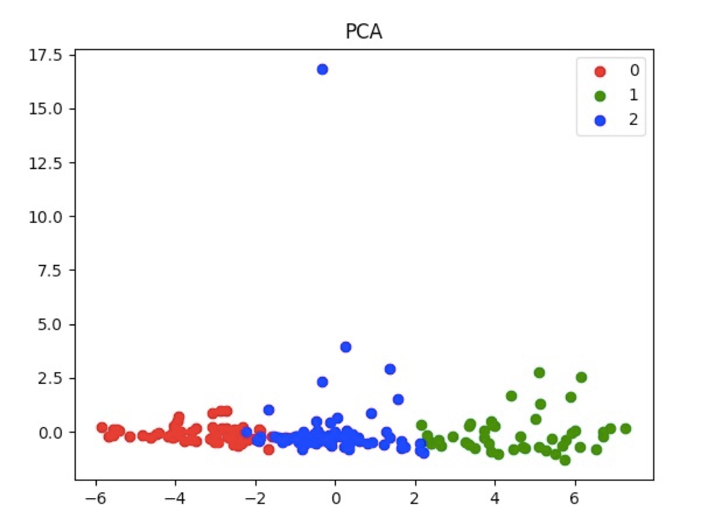
Figure2.Dimensionality reduction with LDA

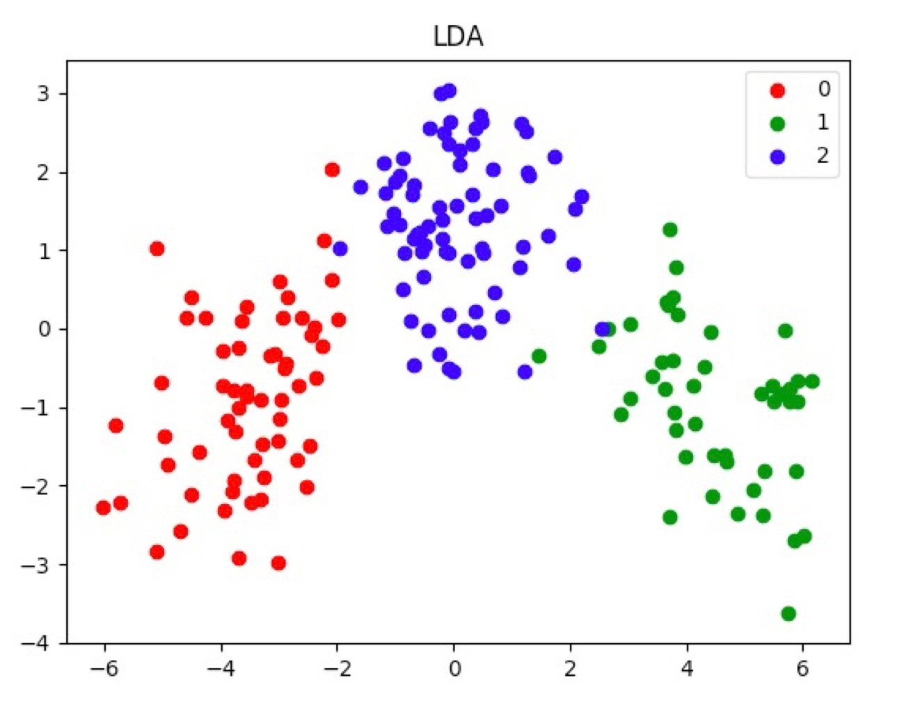
Figure1 shows the result of dimensionality reduction with PCA, which means Principal Component Analysis. All it does is mapping the whole set of data to the coordinate axes that most conveniently represents the set of data, without using any internal classification information in the data. Thus, although it makes the entire set of data more convenient for representation, reduces the number of dimensions and minimizes the loss of information, it may be more difficult to categorize the samples at the same time.

Figure2 shows the result of dimensionality reduction with LDP, which means Linear Discriminant Analysis. That can be clearly seen, after the classification information is added, the three sets of data become more distinguishable. In fact, it simplifies the computation process successfully.

4.2 Results

In our model results, with the method of LDP, we get 2 final dimensions and divide various of countries into 3 categories. Among the figures, class 0 represents fragile countries, class 1 represents stable countries, class 2 represents vulnerable countries.

Table[4-2] The distribution of labels

label	percentage
0: fragile	33.15%
1: vulnerable	41.01%
2: stable	25.84%

5 Logistic Regression Model

5.1 Model Overview

In our model, we aimed at three goals: identifying a country's fragility by analyzing its 21-dimensional data, determining how climate change will affect its fragility and defining the tipping point of climate change when it may push the country to become more fragile.

By selecting 178 sample data from the database of 2014, we can make predictions on the fragility categories of different countries. We analyze 8 different characteristic variables and 1 category variable involved, find out the factors that have the strongest influence on the dependent variable, then we find out a predictable method and evaluate the model, trying to find out the optimal theoretical model to identify the fragility of a country.

Using SPSS and Clementine 12.0 (software), we can have a general understanding of the composition of the dataset by descriptive statistical analysis of it. Then we construct the function of respective variables and dependent variable by making Logistic regression analysis of our dataset, so we can have an intuitive understanding using specific correlation coefficients.

5.2 Details of Logistic Regression Model

We do empirical research by using logistic regression model.
In this case, the event is expressed as label classification, then the probability formula is

$$P(label = 0| X_i) = \frac {e ^{\alpha_0 + \sum \alpha_i x_i}}{1+e ^{\alpha_0 + \sum \alpha_i x_i}}$$

In the formula, $X_i$ represents the model's independent variable, $\alpha_0$ is the constant term, and $\alpha_i$ is the regression coefficient which indicates how much the independent variable affects the probability of the dependent variable.
We can get the expression of the Multinomial Logistic Regression Models by deforming the formula above：

$$ln[\frac{P(label = 1|X_i)}{P(label = 0|X_i)}] = \alpha_0 + \alpha_1 C1 + \alpha_2 C2 + \alpha_3 C3 + \alpha_4 E1 +...$$

$$ln[\frac{P(label = 2|X_i)}{P(label = 0|X_i)}] = \alpha_0 + \alpha_1 C1 + \alpha_2 C2 + \alpha_3 C3 + \alpha_4 E1 +...$$

By using the forward method, we can know the "Variable Importance" of each indicator and get the linear regression model.

5.3 Parameter Setting and Choosing

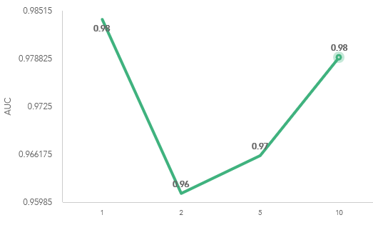
As can be seen from Figure3, when the random seed is 1, the value of AUC is the biggest. So, we choose this parameter to built our model.

Figure3. AUC over Random Seed

5.4 The level of significance of the variable

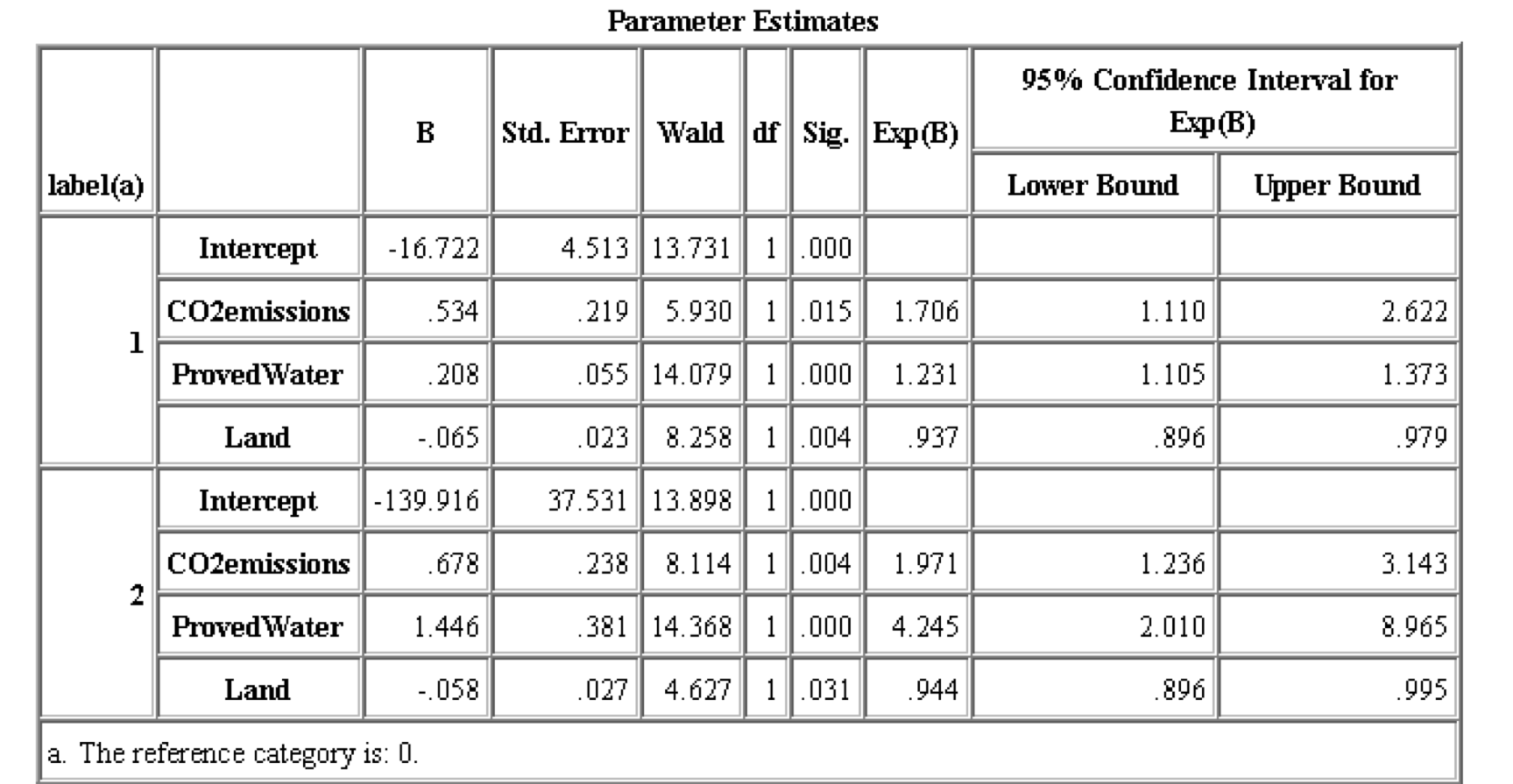
It can be seen from the figure below that the Sig. of Proved Water, Land, and $CO_2$ emissions are less than 0.05, all of them are significant.

Table[5-4] Parameter Estimates

5.5 Results Analysis and Sensitivity Analysis

The final Logistic Regression Model is as follows:

$$ln[\frac {P(label = 2|X_i)}{P(label = 0|X_i)}]= 0.6785*CO_2 emissions+1.446* Proved Water-0.05758*Land -139.9$$

$$ln[\frac {P(label = 1|X_i)}{P(label = 0|X_i)}]= 0.5342*CO_2emissions+0.2082* Proved Water-0.06547*Land -16.72$$

Note that these functions are functions of $label = 1$ and $label = 2$ based on the function of "label = 0"

In the first function:

• When $Proved Water$ increases by 1 unit, the output increases by an average of $0.6785$
• When $CO_2$ emissions increases by 1 unit,the output increases by an average of $2.834$
• When $Land$ increases by 1 unit, the output decreases by an average of $0.05758$

In the second function:

• When $Proved Water$ increases by 1 unit, the output increases by an average of $0.2082$
• When $CO_2$ emissions increases by 1 unit, the output increases by an average of $0.5342$
• When $Land$ increases by 1 unit, the output decreases by an average of $0.06547$

5.6 Some statistical results of the regression

Variable importance：

Table[5-6-1]Values'variable importance in Logistic Regression Model

Value	ProvedWater	$CO_2$ Emissions	Land
Variable importance	0.795	0.106	0.099

Statistic of the effect of the Logistic Regression Model

Table[5-6-2]Statistic of the effect of the Logistic Regression Model

Statistic	Chi_Square	sig	Cox and Snell	Nagelkerke	McFadden
Value	157.546	0	0.746	0.842	0.631

Figure of lift

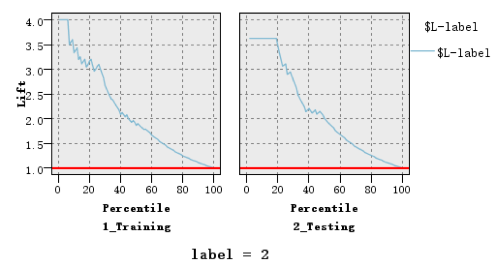
From the right side of the following Figure4, which means the lift of our testing sets, the lift value is much greater than 1 and effect of lift is very well.

Figure4.Lift of 'label=2'

AUC value and accuracy

Using the output of the Clementine software, AUC value is 0.984 on the training set, the correct rate and the error rate are as follows:

Table[5-6-3]Correct rate and Error rate

Partition	1_Training	%	2_Testing	%
Correct	95	82.61%	48	76.19%
Error	20	17.39%	15	23.81%
Total	115		63

5.7 Iraq

In task 2, we choose Iraq, a state in the top 10 list, to analyze the rankings and the changing of feature values, forming Figure5 as follows:

Figure5.The feature indicators' information of Iraq

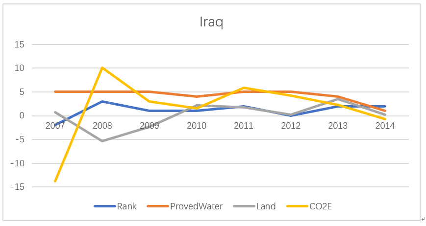
Iraq is one of the fragile countries, whose label is '0'. Combined with the final functions derived from the Logistic Regression Model above, we can analyze the impact of different feature values on Iraq's fragile degree. According to the Logistic Regression Model,we get the functions as follows:

$$ln[\frac {P(label=1)}{P(label=0)}]= 0.5342*CO_2emissions+0.2082* Proved Water-0.06547*Land -16.72$$
$$ln[\frac {P(label=2)}{P(label=0)}]= 0.6785*CO_2emissions+1.446* Proved Water-0.05758*Land -139.9$$

When the $CO_2$ emissions or the Proved Water increases by one unit, the first function produces an average increase of 0.5342 and 0.2082 respectively, which means P(label=1)/[P(label=0)] increasing by $e^{0.5342}$ and $e^{0.2082}$ respectively. When the Land increases by one unit, the first function produces an average decrease of 0.06547, which means P(label=1)/[P(label=0)] decreasing by $e^{0.06547}$.

When the $CO_2$ emissions or the Proved Water increases by one unit, the second function produces an average increase of $0.6785$ and $1.446$ respectively, which means $\frac {P(label=2)}{P(label=0)}$ increasing by $e^{0.6785}$ and $e^{1.446}$ respectively. When the Land increases by one unit, the secong function produces an average decrease of 0.05758, which means $\frac{P(label=2)}{P(label=0)}$ decreasing by $e^{0.05758}$.

On the one hand, with the increase of carbon dioxide emissions, the industry development of the country is proceeding rapidly, leading to an increase in the overall national strength and further increasing the stability of the country. And the abundance of available water guarantees for the quality of life of the people and thus improves the stability of the country. On the other hand, in fact, the increase of land area in Iraq is obtained through the struggle of the armed forces with terrorists, bringing along to the country a war and a more unstable state.

6 C&R Trees

6.1 Details of C&R Trees

Table[6-1] Parameter Settings

Symbol	Parameter
random seed	1
training partition size	67%
testing partition size	33%
maximum surrogates	5
minimum change in impurity	0.0001
Impurity measurement for categorical targets	Twoing

Then we get the figure of C&R Trees as follows:

Figure6.C&R Trees

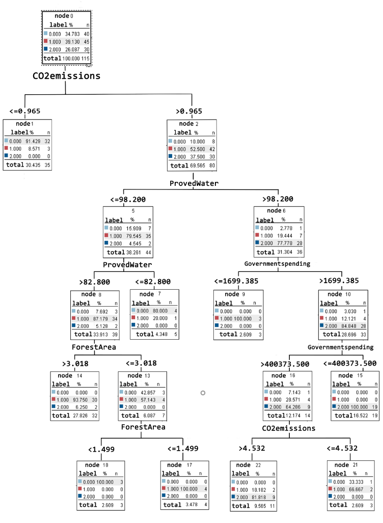
6.2 The Variable Importance of Values

Table [6-2] The Variable importance of values

Values	Variable importance
Temperature change	0.013
Cultivation of Organic Soils	0.013
Land Cover	0.013
Land	0.013
Forest area (% of land area)	0.013
Proved water	0.451
$CO_2$ emissions	0.472
Government Expenditure	0

6.3 Effect Evaluation Statistics

Accuracy

Table[6-3] Accuracy and error rate of C & R Trees model on training set and test set

Partition	1_Training	%	2_Testing	%
Correct	106	90.17%	48	76.19%
Wrong	9	7.83%	15	23.81%}
Total	115		63

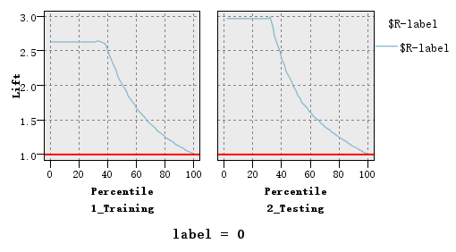
Figure of lift

From the right side of the following figure, which means the lift of our testing sets, the lift value is much greater than 1 and effect of lift is very well.
Figure7. Lift of $label=0$

6.4 Tipping Point

As can be seen from the output of C&R Trees, it is not reliable to predict the fragility of a country with only one indicator. Different indicators interrelate to each other, determining the type of a country together.For example, when a country's $CO_2$ emissions<=0.965, the probability of the label being 0 is 91.429% and being 1 is 8.571%. However, when a country's $CO_2$ emissions>=0.965, more indicators like 'Proved Water', 'Government Spending' and 'Forest Area' should be taken into consideration. We can find more detailed tipping points in the figure of C&R Trees.

Another question is how to predict when a country may reach it. About this, we need to predict this country's information about the environment. To do this we may need Model from other subjects such as Geography or Meteorology. However, without enough data and academic background, it is not easy for us to rein these models. So we may use Time Series Prediction to get the data we need. Then put them into the model we already have(Regression, Tree). After that, we may know after years which label these countries belong to and determine if this country reaches the 'tipping point'.

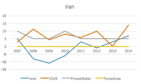
6.5 Iran

In task 3, we choose Iran, a state not in the top 10 list, to predict its fragility, and the specific data in 2014 was listed as follows. Based on the tipping points in C&R Trees, the probability of the label being 0 is 93.750%.When the $CO_2$ emissions<=0.965, climate change may push the country to become more fragile. And the probability is 91.429%. More detailed tipping points of Proved water, Government spending and Forest area can be found in the C&R Trees.

Table[6-5]The specific data of Iran in 2014

Indicator	ProvedWater	$CO_2$ Emissions	ForestArea
Value	96.2	8.28302079	6.564490778

Figure8.The feature indicators' information of Iran

7 Conclusion

7.1 State-Driven Interventions

From the Government Spending data, we choose the proportion of the government spending on environmental protection over the total government spending, p, to measure the ability of a country facing the changing climate. Regardless of extreme natural disasters and geological disasters, once $p > \eta$, we consider that the country has a strong capability to adapt to climate change. Using statistical analysis, we can see the proportions of different countries are as follows:

Figure9. The percentage of the government spending on environmental protection over the total government spending

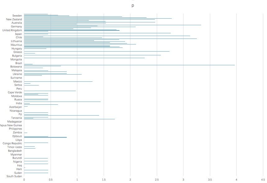
Generally, we choose $\eta = 1$ as a threshold, then the countries with the strong capability to adapt to climate change are as follows:

Georgia, Israel and West Bank, Indonesia, Armenia, Cyprus, Seychelles, Romania, Bulgaria, Greece, Hungary, Latvia, United Arab Emirates, Mauritius, Slovak Republic, Estonia, Italy, Lithuania, Spain, Malta, Poland, Czech Republic, Japan, France, United Kingdom, Slovenia, Belgium, Germany, Netherlands, Canada, Australia, Ireland, Iceland, Luxembourg, New Zealand, Switzerland, Norway

We find out that these countries are basically classified as 'stable'.
As for the effect of the human intervention, there are some ways:

1. Encouraging the development of modernized agriculture production, and increasing the investment to build an agricultural disaster-alert system, we can reduce the sensitivity of agriculture production to the climate change. If the arable land during climate change is guaranteed, we can mitigate the risk of climate change and increase the stability of a country.
2. It is significant to control water pollution to ensure the safety of water, as 'Proved Water' plays an important role in our model. Shutting down the high-polluting industries such as papermaking, printing and dyeing until their pollution treatment can be accepted. In agriculture, it is a good idea to irrigate in a water-saving way.
3. Then we turn to $CO_2$ emissions. Developing public transport may decrease the use of cars greatly. And it's acceptable to limit the production of high-energy-consuming enterprises, then we need to encourage the development of high-tech industry. In addition, we can change the structure of energy use and try cleaner energy. What's more, planting more trees may also have an effect.

Estimating the cost of these measures, we can predict from Environment Protection Cost in government spending.

7.2 Smaller or Larger Ranges

From the description above, we can generally see that our model can work pretty well at the level of nations. As for smaller and larger range such as cities and continents, further consideration is necessary. Since the data we collected are all based on countries, and because of the limit of time and resources, we are not able to collect more comprehensive data of different cities and continents. Even though it seems impossible for us to build specific models for cities and continents, we do have some theoretical analysis based on our current model.

With the development of industrialization and urbanization, the division of labor among different cities in a country is more elaborate. So, it's significant to consider the categories of different cities. Compared with cities with less-urbanization, the arable land of central cities is of no concern since the main source of food is grain imports. At the same time, the population structure, unemployment rate and government revenue of different cities are important. Also, compared with the commercial trade between countries, it turns to be much more convenient between cities because of the shortened geographical distance. Effective and timely financial assistance between cities becomes more possible, which actually enhance the stability of a city with convenient transportation. And for cities with less-industrialization, the local agriculture could be sensitive to the climate change. Since the local agriculture produced the most food supply for the city, we must consider the impacts of climate change on agricultural production. Generally speaking, by changing the weights of different factors in our model, we can modify our model to better analyze the fragility of a city.

Talking about the fragility of a continent, the effect of a certain country is insignificant (except Australia). So, we need to make consideration of the overall situation. First, the climatic conditions of a continent are very important. Since the total level of development decided the living conditions, we also need to consider the level of development of the different continent. Besides, the frequent regional conflicts will increase the fragility of a continent, such as the Korean Peninsula and the Middle East. After introducing these extra factors, our model could be more suitable for analyzing the fragility of a continent.

7.3 Other Extension

Decision trees and regression are both classifiers in our model. And it seems that some integrated learning methods work better than a single decision tree. Using Random Forest algorithm, we can train a number of simple decision trees, classify the sample, then vote on the classification results, and finally take the highest vote as the result of the algorithm. In this way, we can decrease the possibility of over-fitting and under-fitting. In practice, the results of cross-validation show that Random Forest algorithm can improve the accuracy of classification. Although the Random Forest algorithm is not as efficient as a single decision tree, they almost have no difference when the dataset is not large enough.

In addition, we tried to make cross-validation of data from different years. We separately clustered data from two different years, labelled them and trained the classifiers. Then we used the classifier of A year to classify the data from B year and got the accuracy. At the same time, we used the classifier of B year to classify the data from B year and got the accuracy. The comparison between these two accuracies showed that there was not a huge difference. Therefore, we mixed the data from all years and trained the classifier to get our final model.

8 Strength and Weakness

8.1 Strength

1. We analyze the problem based on selecting various indicators and collecting data in authoritative websites so that the models we established is of great inclusiveness.
2. Our models are fairly robust due to our comparison of different ways of modelling and detailed sensitivity analysis.
3. We use the figure of C&R Trees to show the classification process. The outcome is intuitive for us to understand the tipping points.
4. We use a variety of evaluation indicators to make a comparison of different model, making the results more digestible.

8.2 Weakness

1. Although we collect abundance data in different years, some data is incomplete from 2015 to 2017.
2. Limited to time, we do not conduct analysis for the influence of different ways of filling with the missing values. And we choose to fill the missing values with means.
3. About predicting when a country may reach the tipping points, to do this we may need Model from other subjects such as Geography or Meteorology. However, without enough data and academic background, it is not easy for us to rein these models.

Letter

Dear manager:

As the rising frequency of the climate changing, people all over the world are facing the situation that climate change becomes increasingly serious and it will influence regional fragility. This problem is growing into the most rigorous challenge. We want to find the inner relationship between the climate change with the country's fragility, and provide an access to mitigate the risk of climate change.

After analyzing the data from FAO database and World bank database, we build a model to identify the category of a country and calculate the fragility-score of the country. In order to evaluate the influence of climate change, we provided a mathematical function to better explain the importance of each different climate indicators.

In the cases of clustering analysis and dimensionality reduction, we focus on finding the probable clustering centers as the categories of the countries. At the very beginning, we tried to divide the 120 scores into three equal parts. Then we classified these countries based on their fragility-scores. But then we found it's more reasonable to classify these countries using clustering analysis. Also, we were confused about which algorithm should we choose. After evaluating the advantage and disadvantage of different kinds of algorithms, we finally combined the K-means algorithm and the mean-shift algorithm. It actually solved the problem that the clustering centers are uncertain.

Based on the logistic regression model, we find out that the three categories of countries are specially related with the following three indicators: $CO_2$ emissions, Proved Water and Land Use. In this case, we use the model with a better sensitivity to give the precise correlation coefficients.

Furthermore, we build a C&R tree and find out that these different indicators are interrelated with each other. They together decided the category of a country. If the data of Proved Water, $CO_2$ emissions, Forest Area and Government spending was given, we can classify the category of a country and determine whether it reaches the tipping point or not.

Also, using the model above, we can also calculate the proportion of environment-protecting spending over the total government spending. Compared the proportion with the specific threshold, it's possible for us to identify which state driven intervention could mitigate the risk of climate change.

In addition, we make further consideration and provided usable suggestion on modifying our model. By considering the different characteristics and classifications of cities, our model can be applied on a small range better. As for a larger range, some geographical factors and political factors should be considered, then our model can fit better with the situation in real life.

Within all these processes, we build our model based on official data and precise analysis. We provided different models and methods to solve these foreseeable problems. Using our strategy can not only ensure the accuracy of predicting but also help to mitigate the risk of climate change.

Yours sincerely,
Team 87601

Reference

1. "Mean shift: A robust approach toward feature space analysis." D. Comaniciu and P. Meer, IEEE Transactions on Pattern Analysis and Machine Intelligence (2002)
2. Li Cheng, T. Caelli, "Doubly-MRF stereo matching", Acoustics Speech and Signal Processing 2003. Proceedings. (ICASSP '03). 2003 IEEE International Conference on, vol. 3, pp. III-685, 2003, ISSN 1520-6149.
3. "k-means++: The advantages of careful seeding" Arthur, David, and Sergei Vassilvitskii, Proceedings of the eighteenth annual ACM-SIAM symposium on Discrete algorithms, Society for Industrial and Applied Mathematics (2007)
4. Krakowka, A.R., Heimel, N., and Galgano, F. "Modeling Environmenal Security in Sub-Sharan Africa – ProQuest." The Geographical Bulletin, 2012, 53 (1): 21-38.
5. Schwartz, P. and Randall, D. "An Abrupt Climate Change Scenario and Its Implications for United States National Security", October 2003.
6. Marco Franciosi, Giulia Menconi: Multi-dimensional sparse time series: feature extraction
7. wiki Cluster analysis, https://en.wikipedia.org/wiki/Cluster_analysis
8. wiki k-means clustering, https://en.wikipedia.org/wiki/K-means_clustering
9. wiki Dimensionality reduction, https://en.wikipedia.org/wiki/Dimensionality_reduction
10. wiki Logistic regression, https://en.wikipedia.org/wiki/Logistic_regression
11. wiki Decision tree learning, https://en.wikipedia.org/wiki/Decision_tree_learning
12. GLOBAL DATA, http://fundforpeace.org/fsi/data/
13. FAOSTAT, http://www.fao.org/faostat/en/#data
14. World Bank Open Data, https://data.worldbank.org/