EKF-SLAM Project Report

---

SLAM

---

1 EKF Filter design

In this simulation, the robot has a state vector includes 4 states at time $t$.

$$\textbf{x}_t=[x_t, y_t, \phi_t, v_t]$$

x, y are a 2D x-y position, $\phi$ is orientation, and v is velocity. In the code, "xEst" means the state vector. And, $P_t$ is covariace matrix of the state, $Q$ is covariance matrix of process noise, $R$ is covariance matrix of observation noise at time $t$. The robot has a speed sensor and a gyro sensor. So, the input vecor can be used as each time step

$$\textbf{u}_t=[v_t, \omega_t]$$ Also, the robot has a GNSS sensor, it means that the robot can observe x-y position at each time. $$\textbf{z}_t=[x_t,y_t]$$ The input and observation vector includes sensor noise.In the code, "observation" function generates the input and observation vector with noise

2 Motion Model Design

The robot model is

$$\dot{x} = vcos(\phi)$$ $$\dot{y} = vsin((\phi)$$ $$\dot{\phi} = \omega$$
So, the motion model is $$\textbf{x}_{t+1} = F\textbf{x}_t+B\textbf{u}_t$$ where $$\begin{equation*} F= \begin{bmatrix} 1 & 0 & 0 & 0\\ 0 & 1 & 0 & 0\\ 0 & 0 & 1 & 0 \\ 0 & 0 & 0 & 0 \\ \end{bmatrix} \end{equation*}$$

$$\begin{equation*} B= \begin{bmatrix} cos(\phi)dt & 0\\ sin(\phi)dt & 0\\ 0 & dt\\ 1 & 0\\ \end{bmatrix} \end{equation*}$$

$dt$ is a time interval.

Its Jacobian matrix is

$$\begin{equation*} J_F= \begin{bmatrix} \frac{dx}{dx}& \frac{dx}{dy} & \frac{dx}{d\phi} & \frac{dx}{dv}\\ \frac{dy}{dx}& \frac{dy}{dy} & \frac{dy}{d\phi} & \frac{dy}{dv}\\ \frac{d\phi}{dx}& \frac{d\phi}{dy} & \frac{d\phi}{d\phi} & \frac{d\phi}{dv}\\ \frac{dv}{dx}& \frac{dv}{dy} & \frac{dv}{d\phi} & \frac{dv}{dv}\\ \end{bmatrix} \end{equation*}$$

$$\begin{equation*} 　= \begin{bmatrix} 1& 0 & -v sin(\phi)dt & cos(\phi)dt\\ 0 & 1 & v cos(\phi)dt & sin(\phi) dt\\ 0 & 0 & 1 & 0\\ 0 & 0 & 0 & 1\\ \end{bmatrix} \end{equation*}$$

3 Observation Model Design

The robot can get x-y position infomation from GPS. So GPS Observation model is

$$\textbf{z}_{t} = H\textbf{x}_t$$
where
$$\begin{equation*} B= \begin{bmatrix} 1 & 0 & 0& 0\\ 0 & 1 & 0& 0\\ \end{bmatrix} \end{equation*}$$
Its Jacobian matrix is
$$\begin{equation*} J_H= \begin{bmatrix} \frac{dx}{dx}& \frac{dx}{dy} & \frac{dx}{d\phi} & \frac{dx}{dv}\\ \frac{dy}{dx}& \frac{dy}{dy} & \frac{dy}{d\phi} & \frac{dy}{dv}\\ \end{bmatrix} \end{equation*}$$
$$\begin{equation*} =\begin{bmatrix} 1& 0 & 0 & 0\\ 0 & 1 & 0 & 0\\ \end{bmatrix} \end{equation*}$$

4 Extented Kalman Filter Summary

Localization process using Extendted Kalman Filter is

4.1 Predict Steps

$x_{Pred} = Fx_t+Bu_t$
$P_{Pred} = J_FP_t J_F^T + Q$

4.2 Update Steps

$z_{Pred} = Hx_{Pred}$
$y = z - z_{Pred}$
$S = J_H P_{Pred}.J_H^T + R$
$K = P_{Pred}.J_H^T S^{-1}$
$x_{t+1} = x_{Pred} + Ky$
$P_{t+1} = ( I - K J_H) P_{Pred}$

5 Experiments

5.1 Parameter Settings

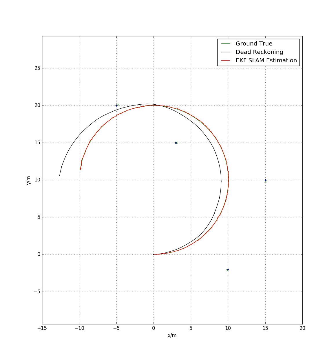
The robot is running at linear speed 1.0 m/s, twist speed is 0.1 rad/s. There are four already known landmark, which are located at (10,-2),(15,10),(3,15),(-5,20). The motion model noise and observation noise are gaussian noise, the mean is 0, the covariance is [0,1].

5.2 Results

In our EKF simulation system, we show the three kind of line results.

• The green line stands for ground true result
• the red stands for ekf-slam estimate result
• the black line stands for dead reckoning(odom data using motion model).
  

5 Appendix: Python Code

"""
Extended Kalman Filter SLAM example
author: Atsushi Sakai (@Atsushi_twi)
"""
import math
import numpy as np
import matplotlib.pyplot as plt
# EKF state covariance
Cx = np.diag([0.5, 0.5, np.deg2rad(30.0)])**2
#  Simulation parameter
Qsim = np.diag([0.2, np.deg2rad(1.0)])**2
Rsim = np.diag([1.0, np.deg2rad(10.0)])**2
DT = 0.1  # time tick [s]
SIM_TIME = 50.0  # simulation time [s]
MAX_RANGE = 20.0  # maximum observation range
M_DIST_TH = 2.0  # Threshold of Mahalanobis distance for data association.
STATE_SIZE = 3  # State size [x,y,yaw]
LM_SIZE = 2  # LM state size [x,y]
show_animation = True
def ekf_slam(xEst, PEst, u, z):
    # Predict
    S = STATE_SIZE
    xEst[0:S] = motion_model(xEst[0:S], u)
    G, Fx = jacob_motion(xEst[0:S], u)
    PEst[0:S, 0:S] = G.T * PEst[0:S, 0:S] * G + Fx.T * Cx * Fx
    initP = np.eye(2)
    # Update
    for iz in range(len(z[:, 0])):  # for each observation
        minid = search_correspond_LM_ID(xEst, PEst, z[iz, 0:2])
        nLM = calc_n_LM(xEst)
        if minid == nLM:
            print("New LM")
            # Extend state and covariance matrix
            xAug = np.vstack((xEst, calc_LM_Pos(xEst, z[iz, :])))
            PAug = np.vstack((np.hstack((PEst, np.zeros((len(xEst), LM_SIZE)))),
                              np.hstack((np.zeros((LM_SIZE, len(xEst))), initP))))
            xEst = xAug
            PEst = PAug
        lm = get_LM_Pos_from_state(xEst, minid)
        y, S, H = calc_innovation(lm, xEst, PEst, z[iz, 0:2], minid)
        K = (PEst @ H.T) @ np.linalg.inv(S)
        xEst = xEst + (K @ y)
        PEst = (np.eye(len(xEst)) - (K @ H)) @ PEst
    xEst[2] = pi_2_pi(xEst[2])
    return xEst, PEst
def calc_input():
    v = 1.0  # [m/s]
    yawrate = 0.1  # [rad/s]
    u = np.array([[v, yawrate]]).T
    return u
def observation(xTrue, xd, u, RFID):
    xTrue = motion_model(xTrue, u)
    # add noise to gps x-y
    z = np.zeros((0, 3))
    for i in range(len(RFID[:, 0])):
        dx = RFID[i, 0] - xTrue[0, 0]
        dy = RFID[i, 1] - xTrue[1, 0]
        d = math.sqrt(dx**2 + dy**2)
        angle = pi_2_pi(math.atan2(dy, dx) - xTrue[2, 0])
        if d <= MAX_RANGE:
            dn = d + np.random.randn() * Qsim[0, 0]  # add noise
            anglen = angle + np.random.randn() * Qsim[1, 1]  # add noise
            zi = np.array([dn, anglen, i])
            z = np.vstack((z, zi))
    # add noise to input
    ud = np.array([[
        u[0, 0] + np.random.randn() * Rsim[0, 0],
        u[1, 0] + np.random.randn() * Rsim[1, 1]]]).T
    xd = motion_model(xd, ud)
    return xTrue, z, xd, ud
def motion_model(x, u):
    F = np.array([[1.0, 0, 0],
                  [0, 1.0, 0],
                  [0, 0, 1.0]])
    B = np.array([[DT * math.cos(x[2, 0]), 0],
                  [DT * math.sin(x[2, 0]), 0],
                  [0.0, DT]])
    x = (F @ x) + (B @ u)
    return x
def calc_n_LM(x):
    n = int((len(x) - STATE_SIZE) / LM_SIZE)
    return n
def jacob_motion(x, u):
    Fx = np.hstack((np.eye(STATE_SIZE), np.zeros(
        (STATE_SIZE, LM_SIZE * calc_n_LM(x)))))
    jF = np.array([[0.0, 0.0, -DT * u[0] * math.sin(x[2, 0])],
                   [0.0, 0.0, DT * u[0] * math.cos(x[2, 0])],
                   [0.0, 0.0, 0.0]])
    G = np.eye(STATE_SIZE) + Fx.T * jF * Fx
    return G, Fx,
def calc_LM_Pos(x, z):
    zp = np.zeros((2, 1))
    zp[0, 0] = x[0, 0] + z[0] * math.cos(x[2, 0] + z[1])
    zp[1, 0] = x[1, 0] + z[0] * math.sin(x[2, 0] + z[1])
    #zp[0, 0] = x[0, 0] + z[0, 0] * math.cos(x[2, 0] + z[0, 1])
    #zp[1, 0] = x[1, 0] + z[0, 0] * math.sin(x[2, 0] + z[0, 1])
    return zp
def get_LM_Pos_from_state(x, ind):
    lm = x[STATE_SIZE + LM_SIZE * ind: STATE_SIZE + LM_SIZE * (ind + 1), :]
    return lm
def search_correspond_LM_ID(xAug, PAug, zi):
    """
    Landmark association with Mahalanobis distance
    """
    nLM = calc_n_LM(xAug)
    mdist = []
    for i in range(nLM):
        lm = get_LM_Pos_from_state(xAug, i)
        y, S, H = calc_innovation(lm, xAug, PAug, zi, i)
        mdist.append(y.T @ np.linalg.inv(S) @ y)
    mdist.append(M_DIST_TH)  # new landmark
    minid = mdist.index(min(mdist))
    return minid
def calc_innovation(lm, xEst, PEst, z, LMid):
    delta = lm - xEst[0:2]
    q = (delta.T @ delta)[0, 0]
    zangle = math.atan2(delta[1, 0], delta[0, 0]) - xEst[2, 0]
    zp = np.array([[math.sqrt(q), pi_2_pi(zangle)]])
    y = (z - zp).T
    y[1] = pi_2_pi(y[1])
    H = jacobH(q, delta, xEst, LMid + 1)
    S = H @ PEst @ H.T + Cx[0:2, 0:2]
    return y, S, H
def jacobH(q, delta, x, i):
    sq = math.sqrt(q)
    G = np.array([[-sq * delta[0, 0], - sq * delta[1, 0], 0, sq * delta[0, 0], sq * delta[1, 0]],
                  [delta[1, 0], - delta[0, 0], - 1.0, - delta[1, 0], delta[0, 0]]])
    G = G / q
    nLM = calc_n_LM(x)
    F1 = np.hstack((np.eye(3), np.zeros((3, 2 * nLM))))
    F2 = np.hstack((np.zeros((2, 3)), np.zeros((2, 2 * (i - 1))),
                    np.eye(2), np.zeros((2, 2 * nLM - 2 * i))))
    F = np.vstack((F1, F2))
    H = G @ F
    return H
def pi_2_pi(angle):
    return (angle + math.pi) % (2 * math.pi) - math.pi
def main():
    print(__file__ + " start!!")
    time = 0.0
    # RFID positions [x, y]
    RFID = np.array([[10.0, -2.0],
                     [15.0, 10.0],
                     [3.0, 15.0],
                     [-5.0, 20.0]])
    # State Vector [x y yaw v]'
    xEst = np.zeros((STATE_SIZE, 1))
    xTrue = np.zeros((STATE_SIZE, 1))
    PEst = np.eye(STATE_SIZE)
    xDR = np.zeros((STATE_SIZE, 1))  # Dead reckoning
    # history
    hxEst = xEst
    hxTrue = xTrue
    hxDR = xTrue
    while SIM_TIME >= time:
        time += DT
        u = calc_input()
        xTrue, z, xDR, ud = observation(xTrue, xDR, u, RFID)
        xEst, PEst = ekf_slam(xEst, PEst, ud, z)
        x_state = xEst[0:STATE_SIZE]
        # store data history
        hxEst = np.hstack((hxEst, x_state))
        hxDR = np.hstack((hxDR, xDR))
        hxTrue = np.hstack((hxTrue, xTrue))
        if show_animation:  # pragma: no cover
            plt.cla()
            plt.plot(RFID[:, 0], RFID[:, 1], "*b", lw='3')
            plt.plot(xEst[0], xEst[1], ".r")
            # plot landmark
            for i in range(calc_n_LM(xEst)):
                plt.plot(xEst[STATE_SIZE + i * 2],
                         xEst[STATE_SIZE + i * 2 + 1], "xg")
            gt,=plt.plot(hxTrue[0, :],
                     hxTrue[1, :], "-g")
            dr,=plt.plot(hxDR[0, :],
                     hxDR[1, :], "-k")
            est,=plt.plot(hxEst[0, :],
                     hxEst[1, :], "-r")
            plt.axis("equal")
            plt.xlabel('x/m')
            plt.ylabel('y/m')
            plt.grid(True)
            plt.legend([gt,dr,est],['Ground True','Dead Reckoning', 'EKF SLAM Estimation'],loc='best')
            plt.pause(0.001)
if __name__ == '__main__':
    main()