@youngwang
2017-12-09T01:31:35.000000Z
字数 4011
阅读 999
Problem 5.1 & 5.2
1. Abstract
- 5.1. Solve for the potential in the prism geometry in Figure 5.4.
- 5.2. Use the symmetry of the problem described in Figure 5.4 to write a program that solves for V by calculating the potential in only half of one quadrant of the x-y plane.
2. Background
2.1 Relaxation (iterative method)
In numerical mathematics, relaxation methods are iterative methods for solving systems of equations, including nonlinear systems.
Relaxation methods were developed for solving large sparse linear systems, which arose as finite-difference discretizations of differential equations. They are also used for the solution of linear equations for linear least-squares problems and also for systems of linear inequalities, such as those arising in linear programming. They have also been developed for solving nonlinear systems of equations.
Relaxation methods are important especially in the solution of linear systems used to model elliptic partial differential equations, such as Laplace's equation and its generalization, Poisson's equation. These equations describe boundary-value problems, in which the solution-function's values are specified on boundary of a domain; the problem is to compute a solution also on its interior. Relaxation methods are used to solve the linear equations resulting from a discretization of the differential equation, for example by finite differences.
These iterative methods of relaxation should not be confused with "relaxations" in mathematical optimization, which approximate a difficult problem by a simpler problem, whose "relaxed" solution provides information about the solution of the original problem.
2.2 Jacobi Method
In numerical linear algebra, the Jacobi method (or Jacobi iterative method) is an algorithm for determining the solutions of a diagonally dominant system of linear equations. Each diagonal element is solved for, and an approximate value is plugged in. The process is then iterated until it converges. This algorithm is a stripped-down version of the Jacobi transformation method of matrix diagonalization. The method is named after Carl Gustav Jacob Jacobi.
3. Main
3.1 Formulation and Algorithm
Here what we need to deal with is the Laplace's equation:
The numerical solution to this equation is :
Assuming the system we investigate is infinite along , thus our problem is transferred into a two-dimensional one, with the solution reducing to:
3.2 Jacobi Method
Mathematically the Jacobi method can be expressed as:
3.3 Results
首先,由于对称性可知,我们可以把场的分布分成四个象限。先画出其中每一个象限的图像:
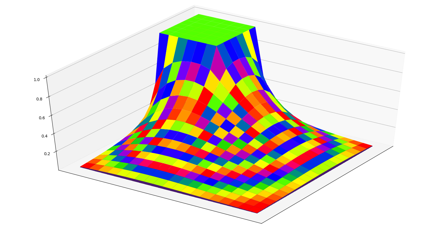
由彩色图很容易看出电场分布
关键代码如下:
while delta_v>0.000005:delta_v=0for i in np.arange(0,7):for j in np.arange(7,20):vn[i][j]=(v0[i-1][j]+v0[i+1][j]+v0[i][j-1]+v0[i][j+1])/4delta_v=delta_v + abs(v0[i][j]-vn[i][j])for i in np.arange(7,20):for j in np.arange(0,20):vn[i][j]=(v0[i-1][j]+v0[i+1][j]+v0[i][j-1]+v0[i][j+1])/4delta_v=delta_v + abs(v0[i][j]-vn[i][j])
接下来我们将四个象限的部分拼接在一起;
关键代码如下:
v1 = np.zeros([41,41])for i in np.arange(0,20):for j in np.arange(0,20):v1[i+20][j+20] = v0[i][j]v1[20-i][20+j] = v0[i][j]v1[20+i][20-j] = v0[i][j]v1[20-i][20-j] = v0[i][j]
这里我们对四个部分分别关于x、y轴对称,巧妙的解决了拼接图案的问题:
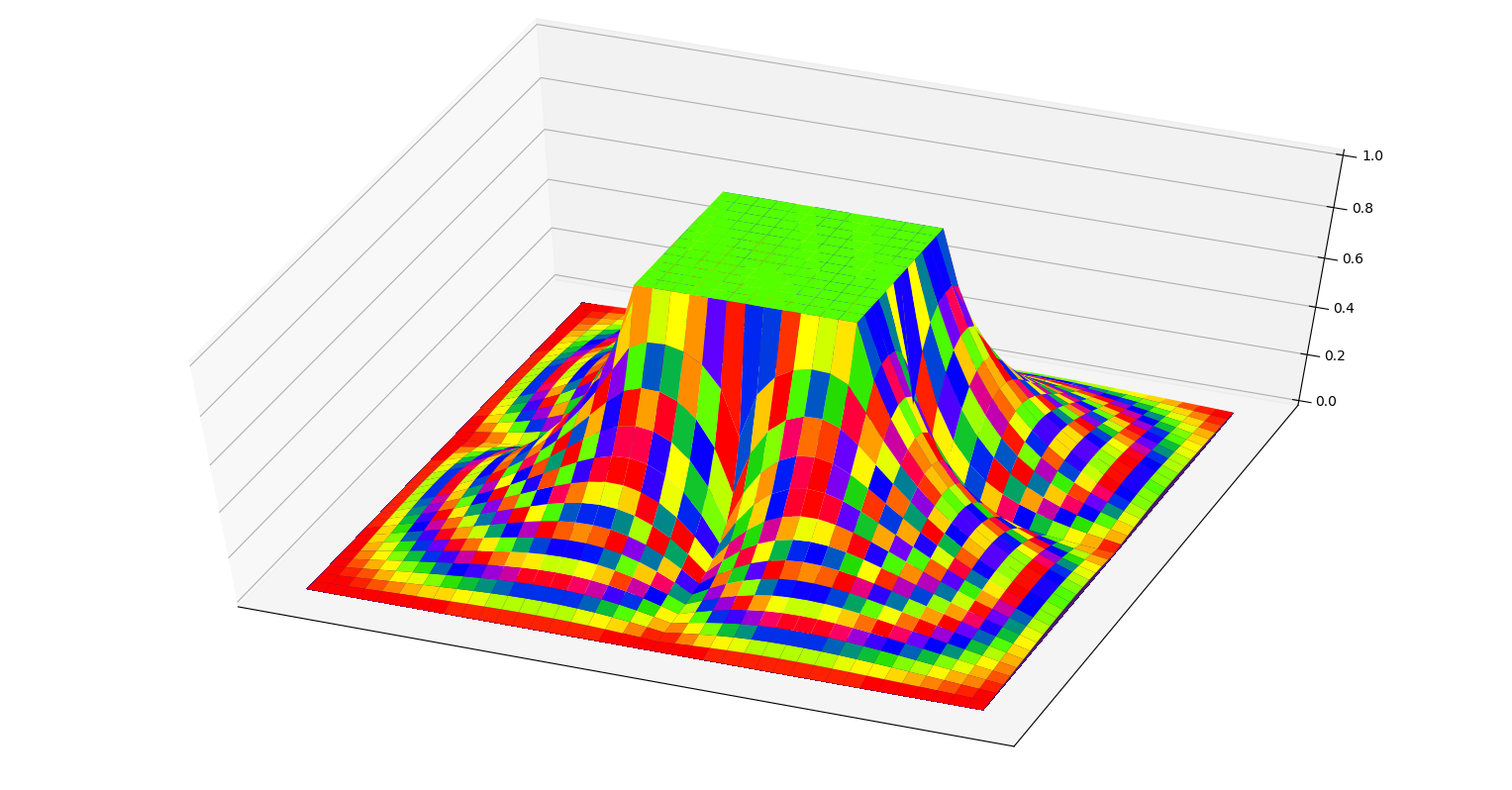
不过,做到这里忽然发现一个很严重的问题。这幅彩图中可以看出,x、y轴附近出现了一道凹下去的部分,就像山谷等高线里凹下去的山谷部分一样。显然这是不符合我们预期的。为什么???
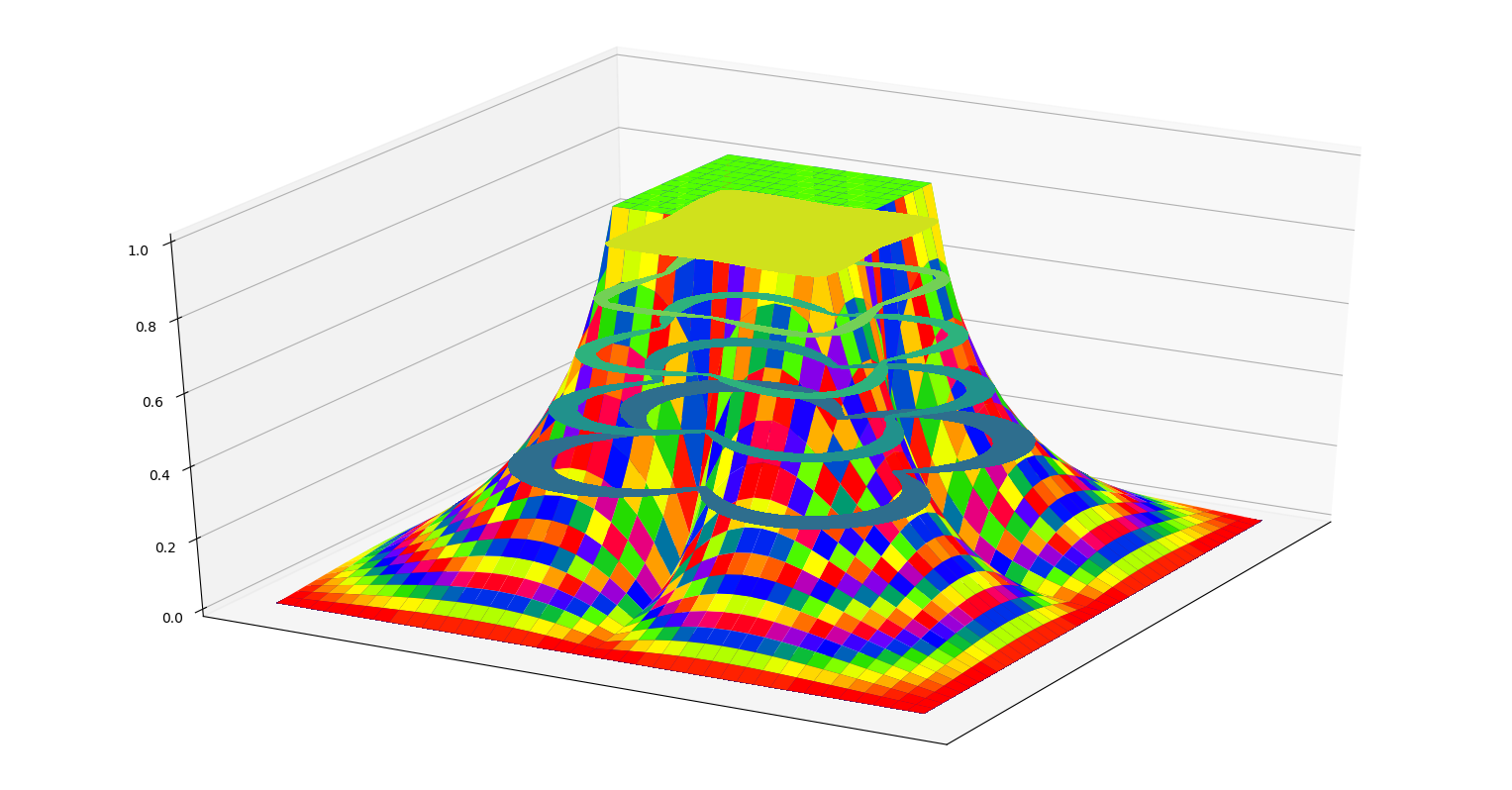
这里通过设置断点的方法,查找最后生成的矩阵,发现x、y轴所在处的值明显和运算公式不符。原因是,在处理第一象限部分时,对于边界的处理过于粗暴——直接套公式然而没有考虑到,当取i(或j)值为0时,(或)是不存在的(没有报错,可能默认为值为0了)
因此加入修正:
while delta_v>0.000005: delta_v=0for i in np.arange(1,7):for j in np.arange(7,20):vn[i][j]=(v0[i-1][j]+v0[i+1][j]+v0[i][j-1]+v0[i][j+1])/4delta_v=delta_v + abs(v0[i][j]-vn[i][j])for i in np.arange(7,20):for j in np.arange(1,20):vn[i][j]=(v0[i-1][j]+v0[i+1][j]+v0[i][j-1]+v0[i][j+1])/4delta_v=delta_v + abs(v0[i][j]-vn[i][j])for j in np.arange(7,20):vn[0][j] = (v0[1][j]*2 + v0[0][j+1] + v0[0][j-1])/4delta_v=delta_v + abs(v0[0][j]-vn[0][j])for i in np.arange(7,20):vn[i][0] = (v0[i][1]*2 + v0[i+1][0] + v0[i-1][0])/4delta_v=delta_v + abs(v0[i][0]-vn[i][0])
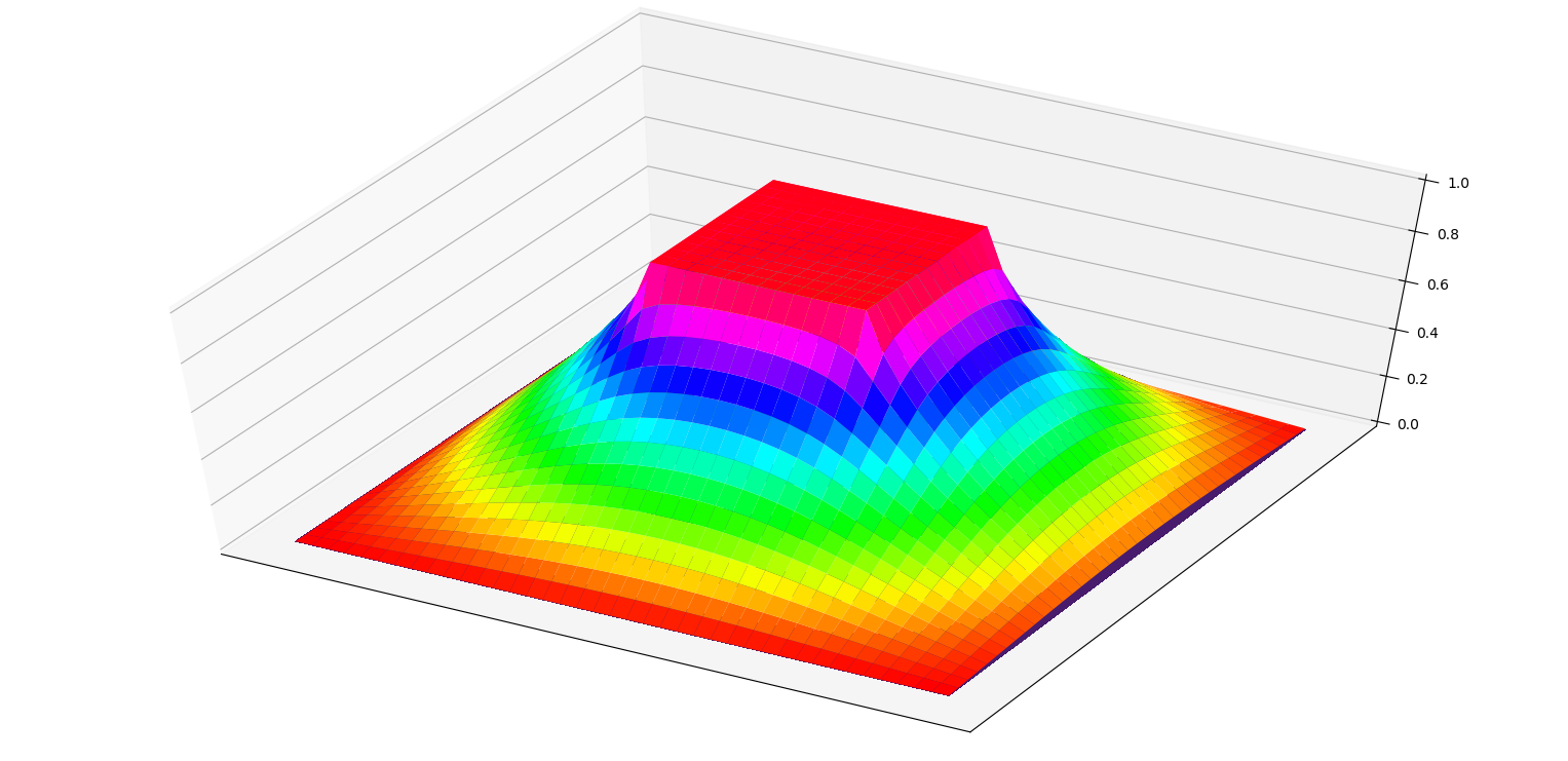
这样画出来的图就对了:
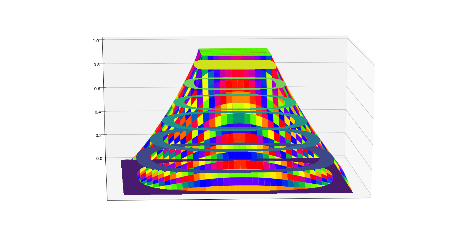
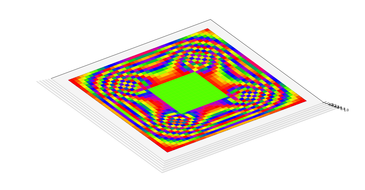
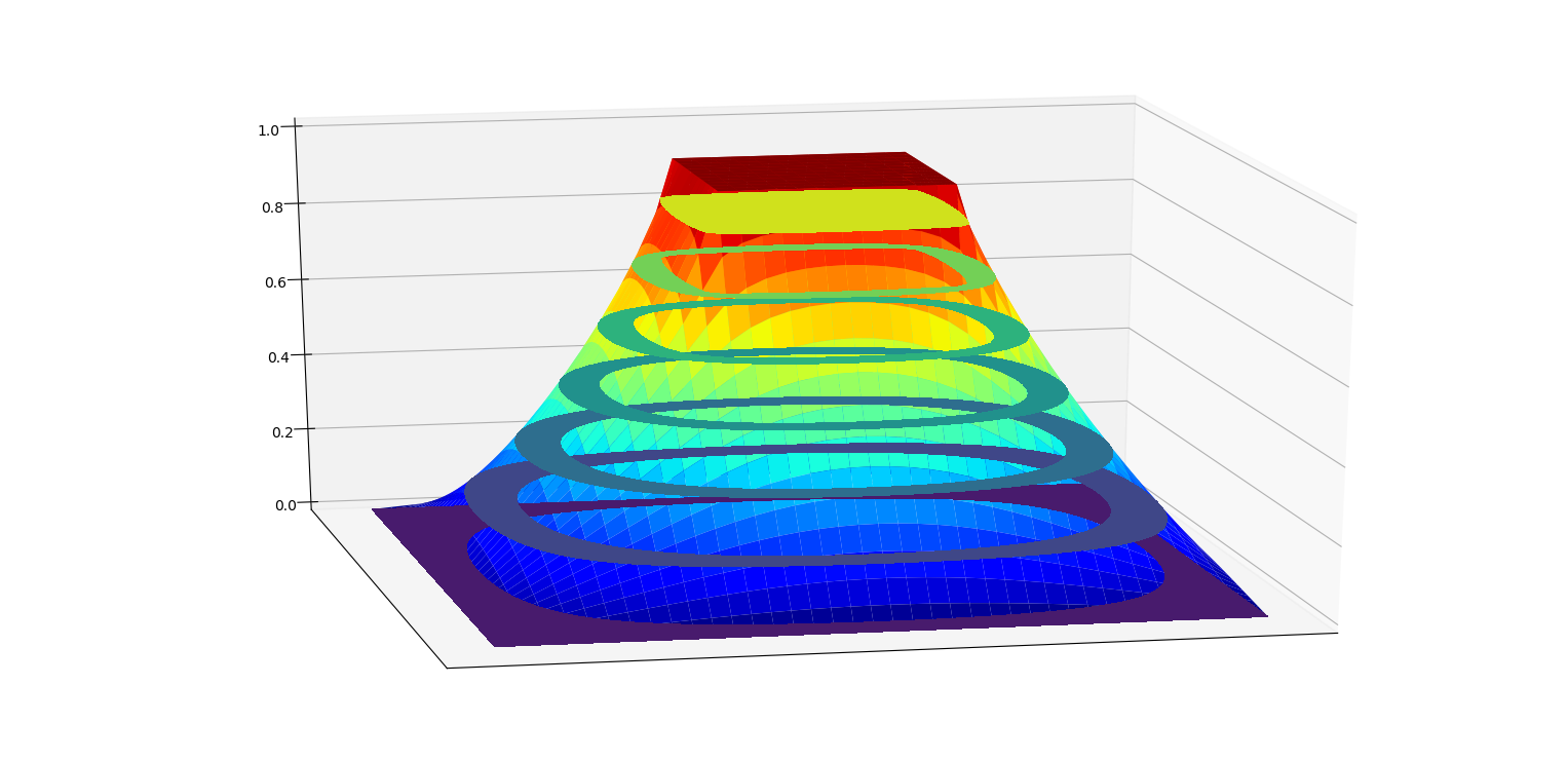
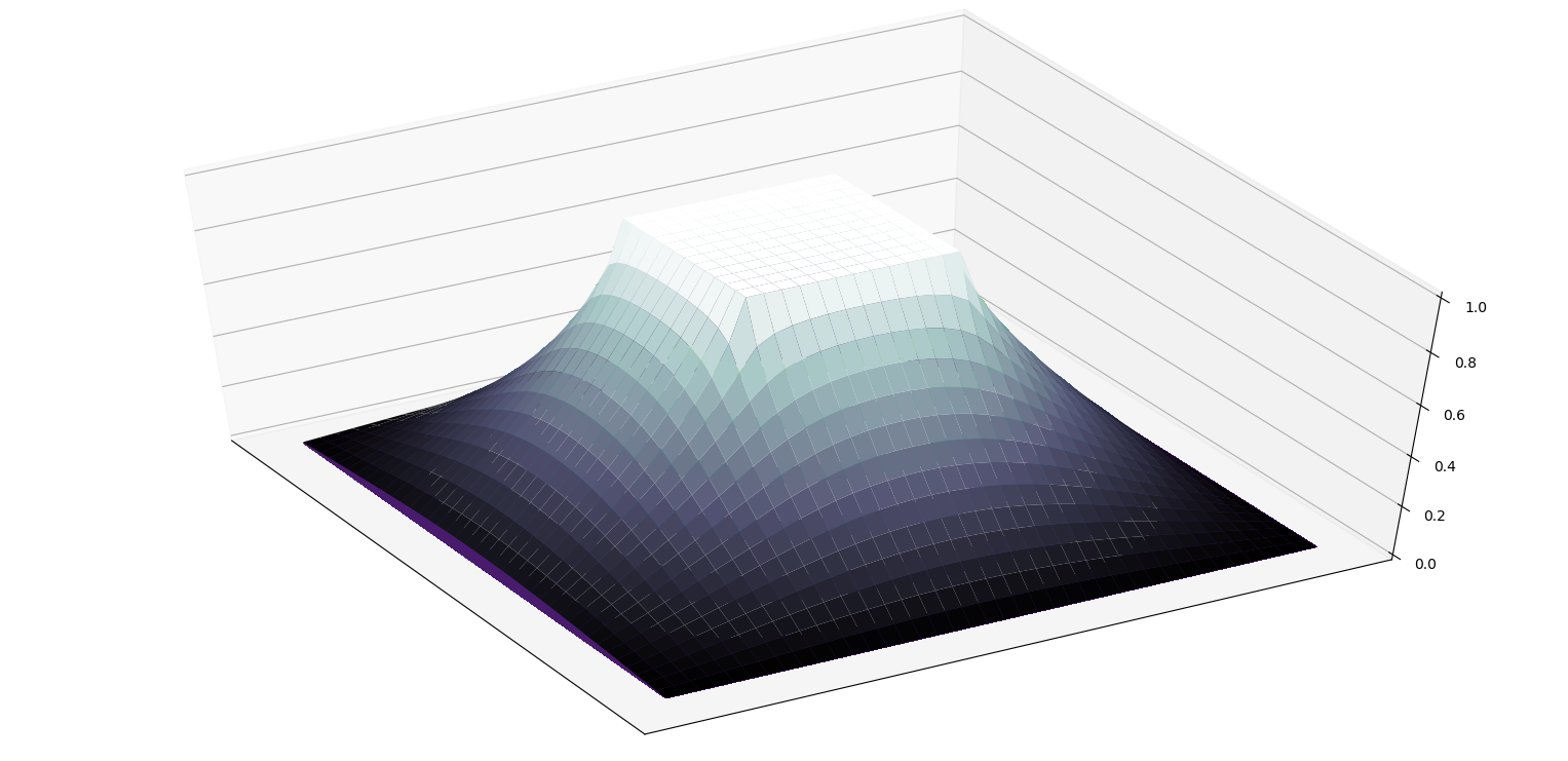
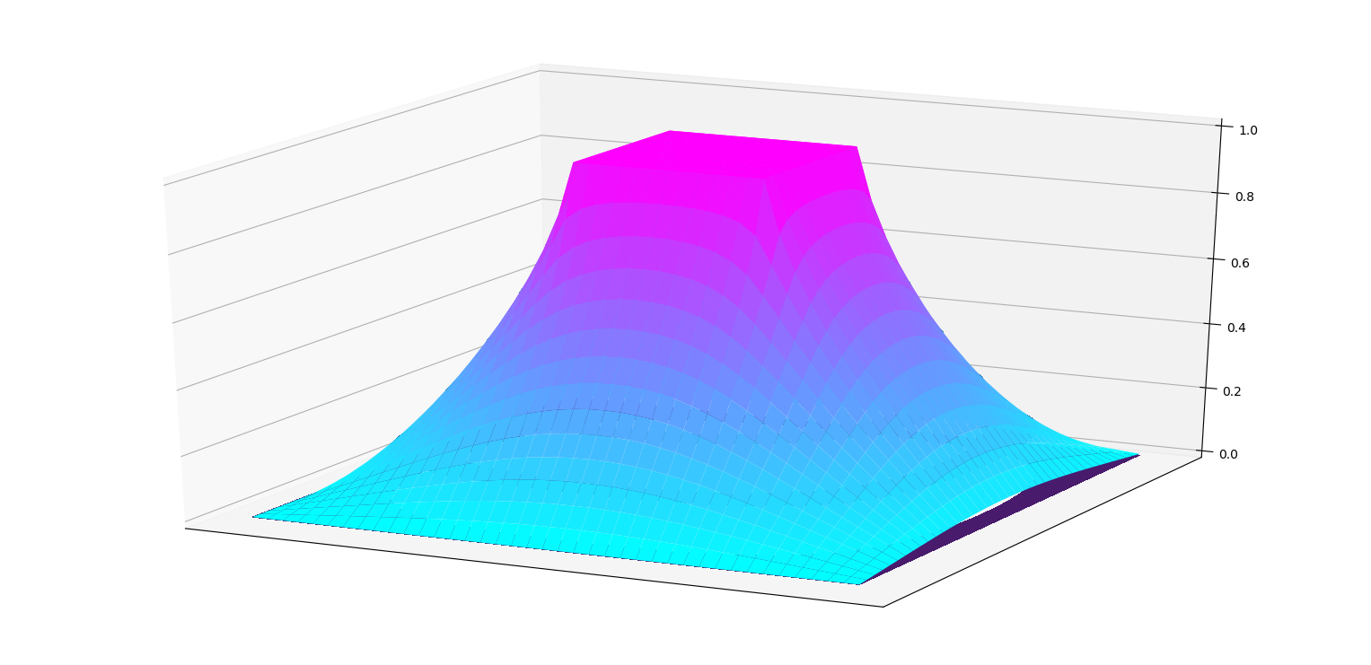
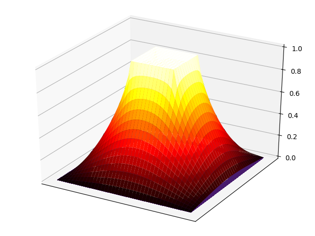
更多3D图像展示:
jet
bone
cool
hsv
hot
4. Acknowledgement
- HollandChen
注:github每到周五晚上就卡的不行,图片传不上去。因此交晚了一点。非常抱歉!
