exercise 07

---

problem 3.13

背景

One example of a simple pendulum is a particle of mass $m$ connected by a massless string to a rigid support.$\theta$ is the angle that the string makes with the verticle.Given the force that the particle beard,the force perpendicular to the string is given by

$$F_{\theta}=-mgsin\theta$$ where $g$ is the acceleration due to gravity.In terms of Newton's second law:$F_{\theta}=md^2s/dt^2$,we assume $\theta$ is always small at the same time,we can obtain the equation of motion $$\frac{d^2\theta}{dt^2}=-\frac gl\theta$$ It has the general solution $$\theta=\theta_0sin(\Omega{t}+\phi)$$ where $\Omega=\sqrt{g/l}$,and $\theta_0$ and $\phi$ are constants that depend on the initial displacement and velocity of the pendulum.
The previous equation describes a frictionless pendulum,we should add some damping.In many cases,this damping force is proportional to the velocity.The equation of motion for our damped pendulum has the form $$\frac{d^2\theta}{dt^2}=-\frac gl\theta-q\frac{d\theta}{dt}$$ .Here $q$ is a parameter that measures the strength of the damping.There are three regimes of distinct physical behaviour.The first regime,called underdamped,occurs for small friction,where the solution $$\theta(t)=\theta_0e^{-qt/2}sin(\sqrt{\Omega^2-q^2/4t}+\phi)$$ At the other extreme,when the damping is large,the behaviour is overdamped,here the solution is $$\theta(t)=\theta_0e^{-(q/2\pm\sqrt{q^2/{4-\Omega^2}})}t$$ At the boundary between the underdamped and overdamped regimes,the pendulum is critically damped with $$\theta(t)=(\theta_0+Ct)e^{-qt/2}$$
Besides the friction,we therefore consider the addition of a driving force to the problem.A convenient choice is to assume that the driving force is sinusoidal with time,with amplitude $F_D$ and angular frequency $\Omega_D$.This leads to the equation of motion $$\frac{d^2\theta}{dt^2}=-\frac gl\theta-q\frac{d\theta}{dt}+F_Dsin(\Omega_Dt)$$ This driving force will pump energy into (or out of) the system.
However,we should have a mumerical method that is suitable for various versions of the pendulum problem.We don't assume the small-angle approximation.Putting all of these ingredients together,we obtain the following equation: $$\frac{d^2\theta}{dt^2}=-\frac glsin(\theta)-q\frac{d\theta}{dt}+F_Dsin(\Omega_Dt)$$ We can rewrite it as two first-order differential equations and obtain
$$\frac{d\omega}{dt}=-\frac glsin(\theta)-q\frac{d\theta}{dt}+F_Dsin(\Omega_Dt)$$ $$\frac{d\theta}{dt}=\omega$$
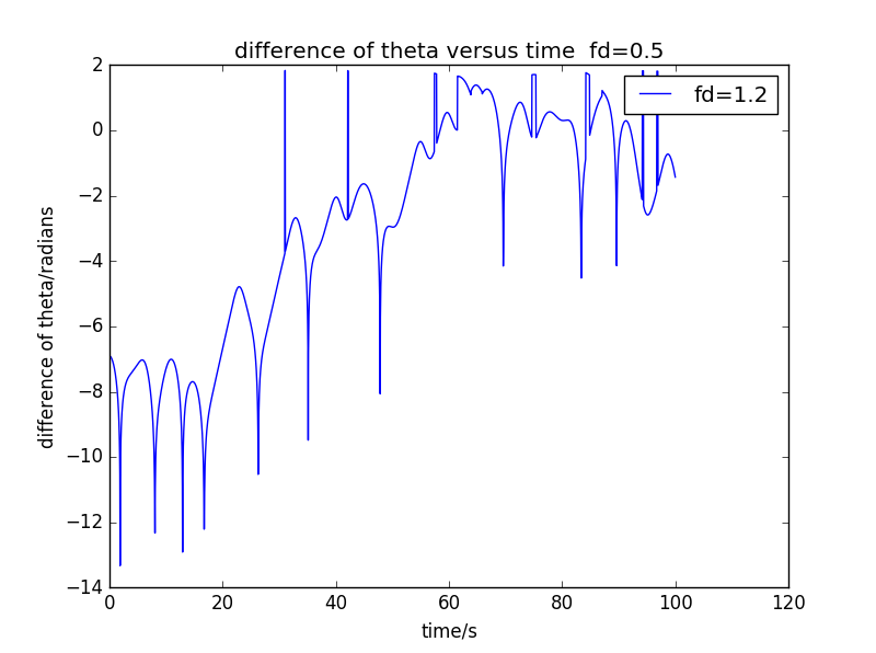
Problem 3.13 need consider the stabilityof the solutions to our problems.We have two identical pendulums with exactly the same lengths and damping factors.The only difference is that we start them with slightly differentinitial angles.Observe the behaviour of the angular positions of two pendulums,$\theta_1$ and $\theta_2$,and the divergence $\Delta\theta=|\theta_1-\theta_2|$.For different values of $F_D$,the trend of the plots vary.This line corresponds to the relation $\log(\Delta\theta)\sim\lambda{t}$,which implies $$\Delta\theta\approx e^{\lambda{t}}$$ The parameter $\lambda$ is known as a Lyapunov exponent.The behaviour of $\Delta\theta$ can be described by a Lyapunov exponent in both the chaotic and nonchaotic regimes.In the former case $\lambda\gt0$,while in the latter,$\lambda\lt0$.The transition to chaos thus occurs when $\lambda=0$.

正文

Code as follows:

import matplotlib.pyplot as plt
import math
class pendulum_1:
    def __init__(self,time_step=0,theta1=0,theta2=0,time_of_duration=0,fd=0.5,q=0.5):
        self.theta1=[theta1]
        self.theta2=[theta2]
        self.dt=time_step
        self.fd=fd
        self.q=q
        self.t=[0]
        self.w1=[0]
        self.w2=[0]
        self.nsteps=int(time_of_duration//time_step+1)
    def calculate(self):
        self.v=[]
        wd=float(2.0/3)
        for i in range(self.nsteps):
            self.w1.append(self.w1[i]+(-math.sin(self.theta1[i])-self.q*self.w1[i]+self.fd*math.sin(wd*self.t[i]))*self.dt)
            self.theta1.append(self.theta1[i]+self.w1[i+1]*self.dt)
            self.w2.append(self.w2[i]+(-math.sin(self.theta2[i])-self.q*self.w2[i]+self.fd*math.sin(wd*self.t[i]))*self.dt)
            self.theta2.append(self.theta2[i]+self.w2[i+1]*self.dt)
            self.t.append(self.t[i]+self.dt)
            self.v=list(map(lambda x:abs(x[0]-x[1]),zip(self.theta1,self.theta2)))
            if self.theta1[i+1]<-math.pi:
                self.theta1[i+1]=self.theta1[i+1]+2*math.pi
            if self.theta1[i+1]>math.pi:
                self.theta1[i+1]=self.theta1[i+1]-2*math.pi
            if self.theta2[i+1]<-math.pi:
                self.theta2[i+1]=self.theta2[i+1]+2*math.pi
            if self.theta2[i+1]>math.pi:
                self.theta2[i+1]=self.theta2[i+1]-2*math.pi
        return 0
    def show_calculate(self,color):
        plt.plot(self.t,self.v,color,label="fd=%r"%(self.fd))
        plt.title('difference of theta versus time  fd=0.5')
        plt.xlabel('time/s')
        plt.ylabel('difference of theta/radians')
        plt.ylim(0,0.001)
a=pendulum_1(0.04,0.200,0.199,60,0,0.5)
a.calculate()
a.show_results('red')
plt.legend()
plt.show()
a=pendulum_1(0.04,0.200,0.199,60,0.5,0.5)
a.calculate()
a.show_results('red')
plt.legend()
plt.show()
a=pendulum_1(0.04,0.200,0.199,60,1.2,0.5)
a.calculate()
a.show_results('red')
plt.legend()
plt.show()

First,draw three plots that behaviours of $\theta$ vary as a function of time for our driven for several different values of the driving force:

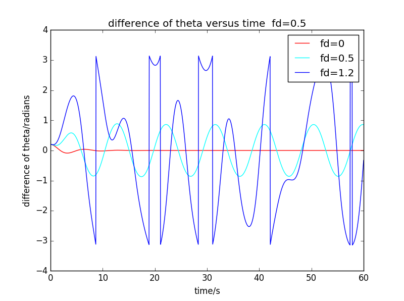
At low drrive,the motion is a simple oscillation.On the other hand,at high drive the motion is chaotic.The behaviour can be both deterministic and unpredictable at the same time.
Next,we consider the behaviour of two,nearly identicle pendulums.The results are as followings:



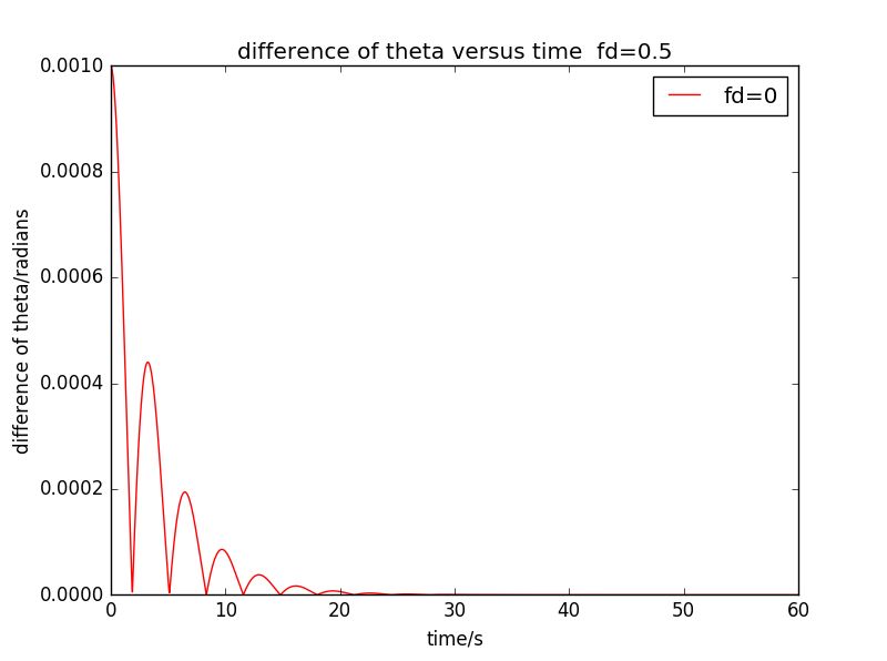
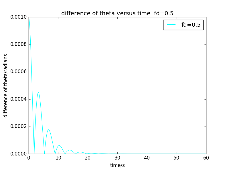
But the y axis'saccuracy isn't enough,the plot can't describe the quality of Lyapunov exponent.I modify the code,and calculate $\log(\Delta{\theta})$ as a function of $t$,so we can obtain the following explicit results:


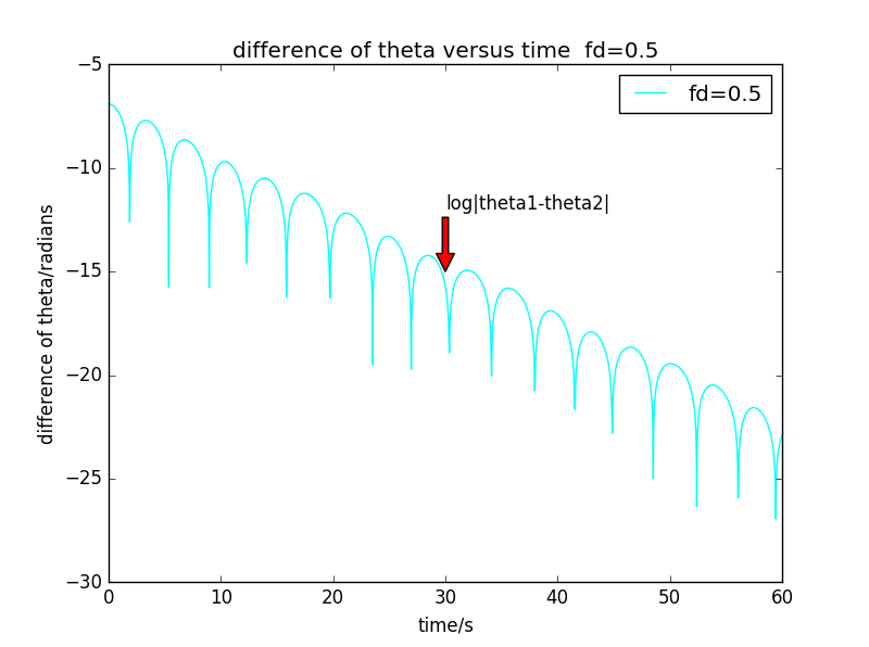
The first figure is plotted in $F_D=0.5$,we can easy to conclude $\log(\Delta{\theta})$ is proportional to $t$,and $\lambda<0$,which represents nonchaotic regimes.This means that the motion of the two pendulums becomes more and more similar,since the difference in the two angles approaches zero as the motion proceeds.
The second figure represents chaotic regimes with $F_D=1.2$ and $\lambda>0$.This is usually described by saying that the two trajectories,$\theta_1(t)$ and $\theta_2(t)$,diverge from one another.This system can obey certain deterministic laws of physics,but still exhibit behaviour that is unpredictable due to an extreme sensititvty to initial conditions.This's the nature of chaotic.
For $F_D=0.5$,we calculate the $\lambda$.Pick up two points from the turning point,such as:(0,-6.78) and (53.7,-20.35),we can obtain the slope:

$$\lambda\approx\frac{-20.35-(-6.78)}{53.7-0}\approx-0.25$$
We can gain the finally equation: $$\Delta\theta\approx{e^{-0.25t}}$$
The second plot is difficulty to find two points,I don't calculate $\lambda$.

致谢

Thanks for the following code(from baidu):

v=list(map(lambda x:x[0]-x[1],zip(v2-v1))