机器学习week5 ex4 review

机器学习 吴恩达

这周的作业主要关于反向传播算法（Backpropagation ,or BP)

1 Neural Networks

在上一次exercise里，我们通过使用神经网络的前馈传播算法（feedforward propagation），利用给定的权重来识别手写的数字。在这一此我们需要通过反向传播算法计算出权重。

1.1 Visualizing the data

脚本文件ex4.m通过调用函数displayData载入数据，并以二维图像的形式展示。（以下代码随机选择其中的100个数字进行展示）

load('ex4data1.mat');
m = size(X, 1);
% Randomly select 100 data points to display
sel = randperm(size(X, 1));
sel = sel(1:100);
displayData(X(sel, :));

这次的数据与上次exercise相同，都是如下图片：

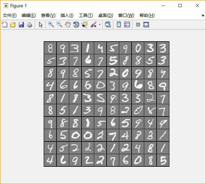
包含了5000个training example，每个training example是一张20*20像素的写有数字的灰度图。每一个像素用一个浮点数表示，代表其灰度的强度。把这个20*20的网格“展开成”一个大小为400的向量，放在矩阵 $X$ 的每一行。

training example的第二部分是一个大小为5000的向量 $y$ ，作为每个 $x$ 的标签。为了适配Octave/MATLAB的下标风格，这里没有0下标："1"-"9"按"1"-"9"标记，而"0"以10标记。

1.2 Model representation

我们的神经网络如下图所示：

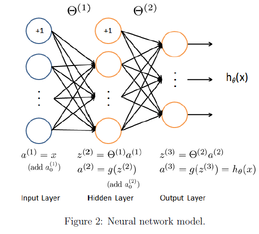
很显然，它具有三个层次：输入层，隐藏层，和输出层。注意到，我们的输入数据是一个数字的图片的像素值，而一张图片共有400个像素，这说明我们的输入层单元有400个（不算偏置单元）。

ex4weights.mat已经给我们提供了一组被训练好的参数($\theta^{(1)}, \theta^{(2)}$)。他们会在ex4.m中被载入到Theta1和Theta2中,并展开成向量形式，合并存入向量nn_params中。Theta1和Theta2的大小被设置为与隐藏层中有25个单元、输出层有10个单元的情况匹配。（也就是说，$\theta_{(1)}$ 的尺寸为 $25\times 401$, 而$\theta^{(2)}$ 的尺寸为 $10 \times 26$)。

ex4.m中这部分代码如下：

% Load the weights into variables Theta1 and Theta2
load('ex4weights.mat');
% Unroll parameters 
nn_params = [Theta1(:) ; Theta2(:)];

这里把Theta1和Theta2展开，存入了一个向量nn_params。

1.3 Feedforward and cost function

现在需要我们为神经网络计算代价函数和梯度。
神经网络的代价函数公式如下（没有经过正规化处理）：

$J(\theta) =\frac{1}{m}\displaystyle{\sum_{i=1}^{m}\sum_{k=1}^{K}[-y_k^{(i)}log(h_{\theta}(x^{(i)}))_k-(1-y_k^{(i)})log(1-(h_{\theta}(x^{(i)}))_k)]}$

之前 $y$ 的标签被定为1-10的整数，为了训练神经网络，我们需要将他们转换成如下向量形式来表示：
$y = \begin{bmatrix} 1 \\ 0 \\ 0 \\ : \\ 0 \end{bmatrix},\begin{bmatrix} 0 \\ 1 \\ 0 \\ : \\ 0 \end{bmatrix}...\begin{bmatrix} 0 \\ 0 \\ 0 \\ : \\ 1 \end{bmatrix}$
这样我们就可以开始计算代价函数了。
完成nnCostFunction中的代码，如下：

% Part 1
% calculate the hypothetical function
a1 = [ones(m,1) X];
z2 = a1 * Theta1';
h1 = sigmoid(z1);
a2 = [ones(size(h1,1),1) h1];
h = sigmoid(a2 * Theta2');
% transform y into vectors
y_vec = eye(num_labels)(y,:);
% then calculate the cost function
J = -1/m * (sum(sum(y_vec.*log(h) + (1-y_vec).*log(1-h))));

• 这里X的第 $i$ 行的转置（$X(i)^T$）才是第 $i$ 个training example。（a1的尺寸为 $5000\times 401$)
  而Theta1和Theta2的第 $i$ 行则存储着z2中第 $i$ 个单元所对应的权重。
  因此，公式中的 $z^{(2)} = \theta^{(1)}a^{(1)}$, 在这里应该表示为z2 = a1*Theta1'。（尺寸为 $5000\times 401$ 的矩阵乘以尺寸为 $401 \times 25$ 的矩阵）。a2和Theta2的部分同理。
• 其中对y的处理部分有一个小技巧。先建立一个10*10的单位矩阵，那么y中值为 $i$ 的数字应转换为其中的第 $i$ 行。

ex4.m中这部分的代码如下:

%% ================ Part 3: Compute Cost (Feedforward) ================
%  To the neural network, you should first start by implementing the
%  feedforward part of the neural network that returns the cost only. You
%  should complete the code in nnCostFunction.m to return cost. After
%  implementing the feedforward to compute the cost, you can verify that
%  your implementation is correct by verifying that you get the same cost
%  as us for the fixed debugging parameters.
%
%  We suggest implementing the feedforward cost *without* regularization
%  first so that it will be easier for you to debug. Later, in part 4, you
%  will get to implement the regularized cost.
%
fprintf('\nFeedforward Using Neural Network ...\n')
% Weight regularization parameter (we set this to 0 here).
lambda = 0;
J = nnCostFunction(nn_params, input_layer_size, hidden_layer_size, ...
                   num_labels, X, y, lambda);
fprintf(['Cost at parameters (loaded from ex4weights): %f '...
         '\n(this value should be about 0.287629)\n'], J);
fprintf('\nProgram paused. Press enter to continue.\n');
pause;

可以看出，这里设置lambda等于0来调用nnCostFunction函数。这暂时还无关紧要，因为我们还没有进行正规化处理。

这时候运行ex4.m：

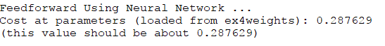
显示结果正确。

1.4 Regularized cost function

经过正规化处理后的代价函数公式如下：
$J(\theta) =\frac{1}{m}\displaystyle{\sum_{i=1}^{m}\sum_{k=1}^{K}[-y_k^{(i)}log(h_{\theta}(x^{(i)}))_k-(1-y_k^{(i)})log(1-(h_{\theta}(x^{(i)}))_k)]} +\\ \frac{\lambda}{2m}[\displaystyle{\sum_{j=1}^{25}\sum_{k=1}^{400}(\theta_{j,k}^{(1)})^2 + \sum_{j=1}^{10}\sum_{k=1}^{25}(\theta_{j,k}^{(2)})^2]}$

以上公式是针对本次练习中的情况写的。说明中特别提到，我们可以仅考虑三层神经网络的情况，但我们的代码必须对各种大小的 $\theta^{(1)}$ 和 $\theta^{(2)}$ 都奏效。
这时候完成nnCostFunction中的这部分代码：

% remember that you don't have to regularize the first column
J = J + lambda/(2*m)*(sum(sum(Theta1(:,2:end).^2))+sum(sum(Theta2(:,2:end).^2)));

在ex4.m中，这部分代码如下：

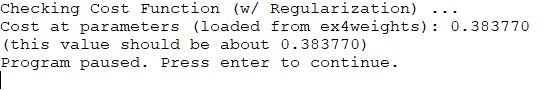
%% =============== Part 4: Implement Regularization ===============
%  Once your cost function implementation is correct, you should now
%  continue to implement the regularization with the cost.
%
fprintf('\nChecking Cost Function (w/ Regularization) ... \n')
% Weight regularization parameter (we set this to 1 here).
lambda = 1;
J = nnCostFunction(nn_params, input_layer_size, hidden_layer_size, ...
                   num_labels, X, y, lambda);
fprintf(['Cost at parameters (loaded from ex4weights): %f '...
         '\n(this value should be about 0.383770)\n'], J);
fprintf('Program paused. Press enter to continue.\n');
pause;

这里lambda被设置为1。

这里要非常注意, $\theta^{(i)}_0$ 是不需要进行正规化的。
如果你不慎忘记了这一点（就像我一样），就会得到下面的错误结果：

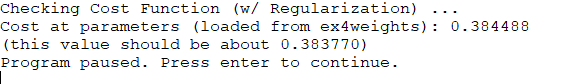
修正之后，得到正确答案：

2. Backpropagation

经过之前的步骤，函数nnCostFunction已经可以返回正确的代价函数 $J$，接下来的步骤我们需要让它能够计算出正确的梯度。

2.1 Sigmoid Gradient

根据公式
$g'(z) = \frac{d}{dz}g(z) = g(z)(1-g(z))$
其中 $g(z) = \frac{1}{1+e^{-z}}$
接下来利用上述公式，完成函数sigmoidGradient。函数需要对 $z$ 是数字、向量、矩阵的情况都奏效。
代码如下：

function g = sigmoidGradient(z)
%SIGMOIDGRADIENT returns the gradient of the sigmoid function
%evaluated at z
%   g = SIGMOIDGRADIENT(z) computes the gradient of the sigmoid function
%   evaluated at z. This should work regardless if z is a matrix or a
%   vector. In particular, if z is a vector or matrix, you should return
%   the gradient for each element.
g = zeros(size(z));
% ====================== YOUR CODE HERE ======================
% Instructions: Compute the gradient of the sigmoid function evaluated at
%               each value of z (z can be a matrix, vector or scalar).
g = sigmoid(z) .* (1 - sigmoid(z))
% =============================================================
end

ex4.m中对这部分的检验代码如下：

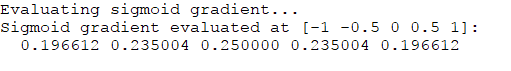
%% ================ Part 5: Sigmoid Gradient  ================
%  Before you start implementing the neural network, you will first
%  implement the gradient for the sigmoid function. You should complete the
%  code in the sigmoidGradient.m file.
%
fprintf('\nEvaluating sigmoid gradient...\n')
g = sigmoidGradient([-1 -0.5 0 0.5 1]);
fprintf('Sigmoid gradient evaluated at [-1 -0.5 0 0.5 1]:\n  ');
fprintf('%f ', g);
fprintf('\n\n');
fprintf('Program paused. Press enter to continue.\n');
pause;

可以看出，它检验的是矩阵 $y = \begin{bmatrix} -1 ,-0.5,0,0.5,1 \end{bmatrix}$。
得到结果如下：

2.2 Random initialization

在使用fminunc等高级优化算法时，我们需要提供一个 $\theta$ 的初始值。如果我们像往常一样以零矩阵为初始，会导致每一层神经网络的不同单元相同。利用反向传播算法后，计算得到的偏导数也相同。也就是说，整个过程中，他们始终会保持相同。这是不符合要求的。

因此我们需要进行随机初始化。
采取的做法是使 $\theta_{ij}$ 处在 $[-\epsilon, \epsilon]$ 的范围上。
约定 $\epsilon = 0.12$。（一般的方法是根据 $\epsilon = \frac{\sqrt{6}}{\sqrt{L_{out} + L_{in}}}$ 来得到 $\epsilon$。）
完成randInitializeWeights中的代码如下：

function W = randInitializeWeights(L_in, L_out)
%RANDINITIALIZEWEIGHTS Randomly initialize the weights of a layer with L_in
%incoming connections and L_out outgoing connections
%   W = RANDINITIALIZEWEIGHTS(L_in, L_out) randomly initializes the weights 
%   of a layer with L_in incoming connections and L_out outgoing 
%   connections. 
%
%   Note that W should be set to a matrix of size(L_out, 1 + L_in) as
%   the first column of W handles the "bias" terms
%
% You need to return the following variables correctly 
W = zeros(L_out, 1 + L_in);
% ====================== YOUR CODE HERE ======================
% Instructions: Initialize W randomly so that we break the symmetry while
%               training the neural network.
%
% Note: The first column of W corresponds to the parameters for the bias unit
%
% Randomly initialize the weights to small values
epsilon_init = 0.12;
W = rand(L_out, 1 + L_in) * 2 * epsilon_init - epsilon_init；
% =========================================================================
end

在ex4.m中这部分代码如下：

%% ================ Part 6: Initializing Pameters ================
%  In this part of the exercise, you will be starting to implment a two
%  layer neural network that classifies digits. You will start by
%  implementing a function to initialize the weights of the neural network
%  (randInitializeWeights.m)
fprintf('\nInitializing Neural Network Parameters ...\n')
initial_Theta1 = randInitializeWeights(input_layer_size, hidden_layer_size);
initial_Theta2 = randInitializeWeights(hidden_layer_size, num_labels);
% Unroll parameters
initial_nn_params = [initial_Theta1(:) ; initial_Theta2(:)];

初始化完成后，再将Theta1和Theta2展开存入一个向量中。

2.3 Backpropagation

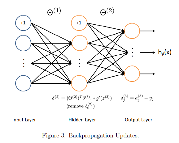
按照上面两张图所示的步骤，我们实现反向传播算法的步骤大致如下：
使用一个对i = 1：m的for循环，i表示的是training example的编号，即 $(x^{(i)},y^{(i)})$。
在每次循环中，
1. 设置输入层 $a^{(1)} = x^{(i)}$。使用前向传播，计算出 $(z^{(2)},a^{(2)},z^{(3)},a^{(3)})$。$a^{(1)}$ 和 $a^{(2)}$ 应该添加偏置单元。
2. 对输出层的每个单元（编号为 $k$ ), 令 $\delta_k^{(3)} = (a_k^{(3)} - y_k)$ ，其中 $y_k = \{0,1\}$,代表当前training example是否是第 $k$ 类。
3. 对于第二层（隐藏层）， 令 $\delta^{(2)} = (\theta^{(2)})\delta^{(3)}.*g'(z^{(2)})$。而输入层不存在误差。
4. 累加以计算梯度（注意要去掉 $\delta^{(2)}_0$):
$\Delta^{(l)} = \Delta^{(l)} + \delta^{(l+1)}(a^{(l)})^T$
5. 计算（未经正规化的）神经网络的梯度如下：$\frac{\partial}{\partial \theta_{ij}^{(l)}}J(\theta) = D_{ij}^{(l)} = \frac{1}{m}\Delta_{ij}^{(l)}$

这部分代码如下：

% Part 2
d3 = h - y_vec;                                             
d2 = (d3*Theta2)(:,2:end).* sigmoidGradient(z2);     
D1 = d2' * a1;    
D2 = d3' * a2;    
Theta1_grad = Theta1_grad + (1/m) * D1;
Theta2_grad = Theta2_grad + (1/m) * D2;

ex4.m中对这部分的检验代码：

%% =============== Part 7: Implement Backpropagation ===============
%  Once your cost matches up with ours, you should proceed to implement the
%  backpropagation algorithm for the neural network. You should add to the
%  code you've written in nnCostFunction.m to return the partial
%  derivatives of the parameters.
%
fprintf('\nChecking Backpropagation... \n');
%  Check gradients by running checkNNGradients
checkNNGradients;
fprintf('\nProgram paused. Press enter to continue.\n');
pause;

其中checkNNGradient是为我们提供的检验梯度的函数。

运行后结果如下：

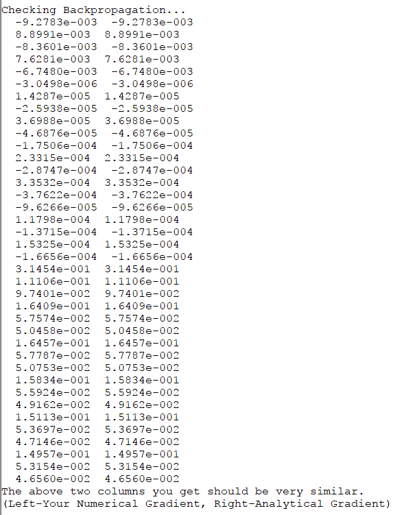
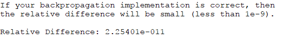
和正确答案相符。并且与gradient checking求出的差异很小：

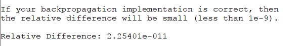
2.4 Gradient checking

Gradient checking是用于对反向传播算法计算结果的检验。用如下方法计算：

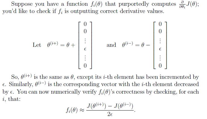
实现代码如下：

function numgrad = computeNumericalGradient(J, theta)
%COMPUTENUMERICALGRADIENT Computes the gradient using "finite differences"
%and gives us a numerical estimate of the gradient.
%   numgrad = COMPUTENUMERICALGRADIENT(J, theta) computes the numerical
%   gradient of the function J around theta. Calling y = J(theta) should
%   return the function value at theta.
% Notes: The following code implements numerical gradient checking, and 
%        returns the numerical gradient.It sets numgrad(i) to (a numerical 
%        approximation of) the partial derivative of J with respect to the 
%        i-th input argument, evaluated at theta. (i.e., numgrad(i) should 
%        be the (approximately) the partial derivative of J with respect 
%        to theta(i).)
%                
numgrad = zeros(size(theta));
perturb = zeros(size(theta));
e = 1e-4;
for p = 1:numel(theta)
    % Set perturbation vector
    perturb(p) = e;
    loss1 = J(theta - perturb);
    loss2 = J(theta + perturb);
    % Compute Numerical Gradient
    numgrad(p) = (loss2 - loss1) / (2*e);
    perturb(p) = 0;
end
end

2.5 Regularized neural networks

正规化后的偏导数公式如下：
$\frac{\partial}{\partial\theta_{ij}^{(l)}} J(\theta) = D_{ij}^{(l)} = \frac{1}{m}\Delta_{ij}^{(l)}$ $(j = 0)$
$\frac{\partial}{\partial\theta_{ij}^{(l)}} J(\theta) = D_{ij}^{(l)} = \frac{1}{m}\Delta_{ij}^{(l)}+ \frac{\lambda}{m}\theta_{ij}^{(l)}$ $(j \geq 1)$

只需增加如下代码：

% Part 3
Theta1_grad(:,2:end) = Theta1_grad(:,2:end) + (lambda/m)*(Theta1(:,2:end));
Theta2_grad(:,2:end) = Theta2_grad(:,2:end) + (lambda/m)*(Theta2(:,2:end));

ex4.m中这部分检验代码：

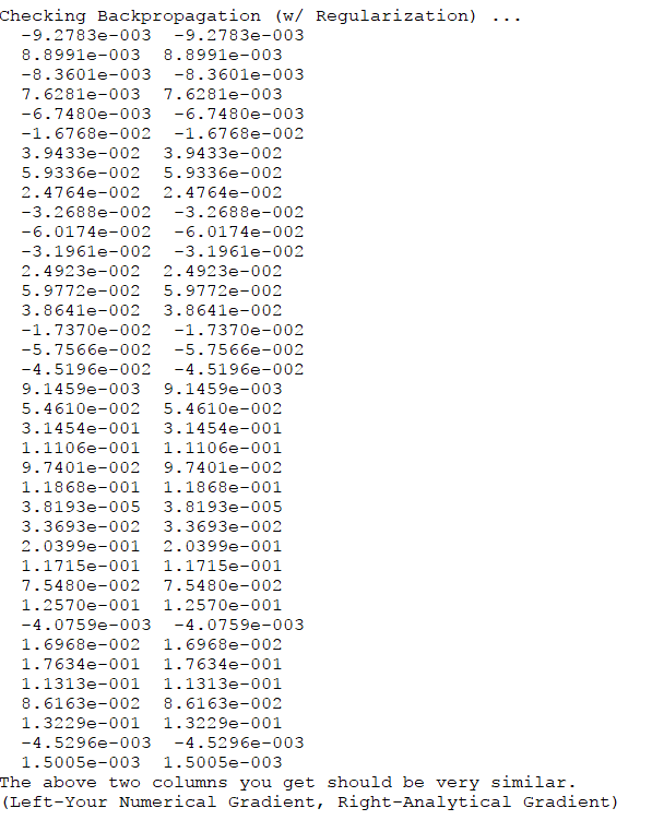
%% =============== Part 8: Implement Regularization ===============
%  Once your backpropagation implementation is correct, you should now
%  continue to implement the regularization with the cost and gradient.
%
fprintf('\nChecking Backpropagation (w/ Regularization) ... \n')
%  Check gradients by running checkNNGradients
lambda = 3;
checkNNGradients(lambda);
% Also output the costFunction debugging values
debug_J  = nnCostFunction(nn_params, input_layer_size, ...
                          hidden_layer_size, num_labels, X, y, lambda);
fprintf(['\n\nCost at (fixed) debugging parameters (w/ lambda = %f): %f ' ...
         '\n(for lambda = 3, this value should be about 0.576051)\n\n'], lambda, debug_J);
fprintf('Program paused. Press enter to continue.\n');
pause;

注意到这里checkNNGradient函数这里带上了参数lambda。这里它被设置为3.
因为在该函数里可以看到如下部分：

if ~exist('lambda', 'var') || isempty(lambda)
    lambda = 0;
end

可以看到不输入参数时，lambda被设置为0。
再次检验可以看出，结果依然正确。

2.6 Learning parameters using fmincg

计算完成后，将training example代入检验准确率。一般来说，准确率大概在95.3%左右。
ex4.m中这部分代码如下：

%% =================== Part 8: Training NN ===================
%  You have now implemented all the code necessary to train a neural 
%  network. To train your neural network, we will now use "fmincg", which
%  is a function which works similarly to "fminunc". Recall that these
%  advanced optimizers are able to train our cost functions efficiently as
%  long as we provide them with the gradient computations.
%
fprintf('\nTraining Neural Network... \n')
%  After you have completed the assignment, change the MaxIter to a larger
%  value to see how more training helps.
options = optimset('MaxIter', 50);
%  You should also try different values of lambda
lambda = 1;
% Create "short hand" for the cost function to be minimized
costFunction = @(p) nnCostFunction(p, ...
                                   input_layer_size, ...
                                   hidden_layer_size, ...
                                   num_labels, X, y, lambda);
% Now, costFunction is a function that takes in only one argument (the
% neural network parameters)
[nn_params, cost] = fmincg(costFunction, initial_nn_params, options);
% Obtain Theta1 and Theta2 back from nn_params
Theta1 = reshape(nn_params(1:hidden_layer_size * (input_layer_size + 1)), ...
                 hidden_layer_size, (input_layer_size + 1));
Theta2 = reshape(nn_params((1 + (hidden_layer_size * (input_layer_size + 1))):end), ...
                 num_labels, (hidden_layer_size + 1));
fprintf('Program paused. Press enter to continue.\n');
pause;

按照迭代次数50次，lambda设置为1来计算，得到如下结果：

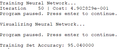
基本吻合。

3 Visualizing the hidden layer

输出隐藏层图形。

3.1 Optional exercise

如果未经正规化，可能会出现overfit的情况：对于training examples可能非常吻合，却不一定适用于新出现的情况。
我们把lambda设置得很小，迭代次数设置得很大，就容易出现这样的情况。
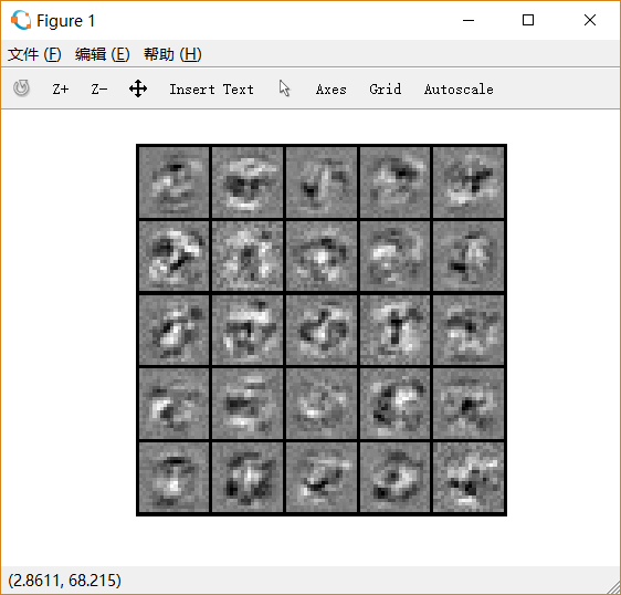
迭代次数：50， lambda=1，如下图：

迭代次数：400， lambda=1， 如下图：

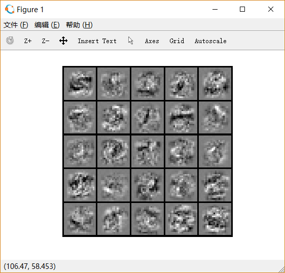
迭代次数：700， lambda=0.1, 如下图：

后两次的training accuracy都接近100%。