机器学习week8 ex7 review

机器学习 吴恩达

这周学习K-means,并将其运用于图片压缩。

1 K-means clustering

先从二维的点开始，使用K-means进行分类。

1.1 Implement K-means

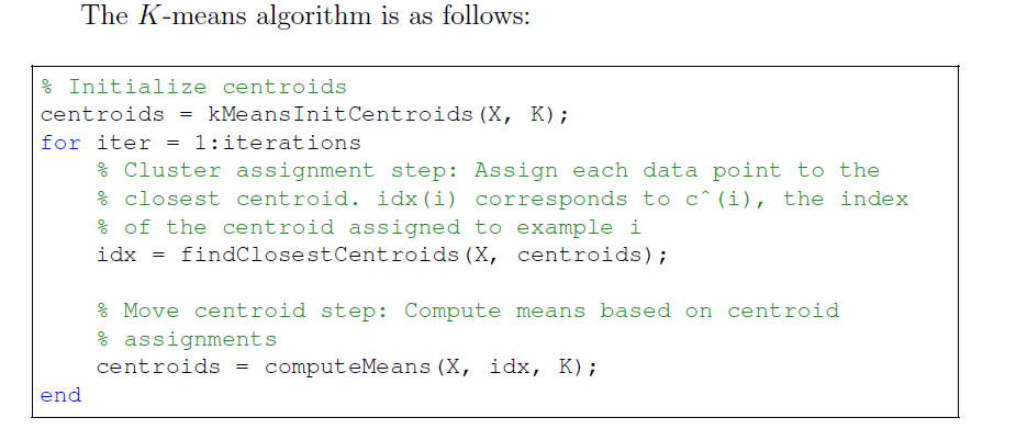
K-means步骤如上，在每次循环中，先对所有点更新分类，再更新每一类的中心坐标。

1.1.1 Finding closest centroids

对每个example，根据公式：

找到距离它最近的centroid，并标记。若有数个距离相同且均为最近，任取一个即可。
代码如下：

function idx = findClosestCentroids(X, centroids)
%FINDCLOSESTCENTROIDS computes the centroid memberships for every example
%   idx = FINDCLOSESTCENTROIDS (X, centroids) returns the closest centroids
%   in idx for a dataset X where each row is a single example. idx = m x 1 
%   vector of centroid assignments (i.e. each entry in range [1..K])
%
% Set K
K = size(centroids, 1);
% You need to return the following variables correctly.
idx = zeros(size(X,1), 1);
% ====================== YOUR CODE HERE ======================
% Instructions: Go over every example, find its closest centroid, and store
%               the index inside idx at the appropriate location.
%               Concretely, idx(i) should contain the index of the centroid
%               closest to example i. Hence, it should be a value in the 
%               range 1..K
%
% Note: You can use a for-loop over the examples to compute this.
%
for i = 1:size(X,1)
  dist = pdist([X(i,:);centroids])(:,1:K);
  [row, col] = find(dist == min(dist));
  idx(i) = col(1);
end;

1.1.2 Compute centroid means

对每个centroid，根据公式：

求出该类所有点的平均值（即中心点）进行更新。
代码如下：

function centroids = computeCentroids(X, idx, K)
%COMPUTECENTROIDS returns the new centroids by computing the means of the 
%data points assigned to each centroid.
%   centroids = COMPUTECENTROIDS(X, idx, K) returns the new centroids by 
%   computing the means of the data points assigned to each centroid. It is
%   given a dataset X where each row is a single data point, a vector
%   idx of centroid assignments (i.e. each entry in range [1..K]) for each
%   example, and K, the number of centroids. You should return a matrix
%   centroids, where each row of centroids is the mean of the data points
%   assigned to it.
%
% Useful variables
[m n] = size(X);
% You need to return the following variables correctly.
centroids = zeros(K, n);
% ====================== YOUR CODE HERE ======================
% Instructions: Go over every centroid and compute mean of all points that
%               belong to it. Concretely, the row vector centroids(i, :)
%               should contain the mean of the data points assigned to
%               centroid i.
%
% Note: You can use a for-loop over the centroids to compute this.
%
for i = 1:K
  centroids(i,:) = mean(X(find(idx == i),:));
end;
% =============================================================
end

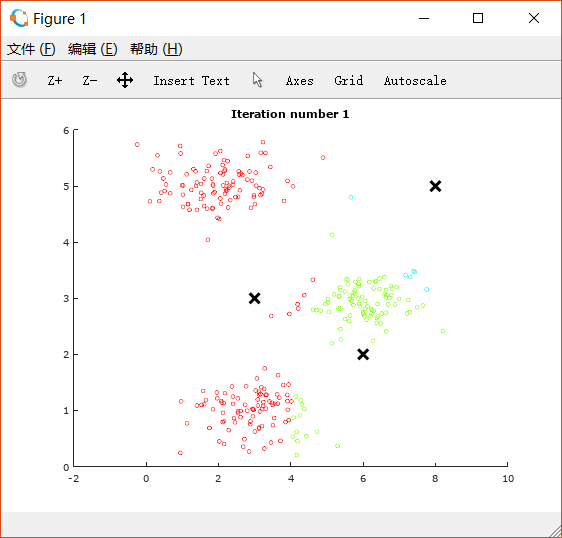
1.2 K-means on example dataset

ex7.m中提供了一个例子，其中中 K 已经被手动初始化过了。

% Settings for running K-Means
K = 3;
max_iters = 10;
% For consistency, here we set centroids to specific values
% but in practice you want to generate them automatically, such as by
% settings them to be random examples (as can be seen in
% kMeansInitCentroids).
initial_centroids = [3 3; 6 2; 8 5];

如上，我们要把点分成三类，迭代次数为10次。三类的中心点初始化为$(3,3),(6,2),(8,5)$.
得到如下图像。（中间的图像略去，只展示开始和完成时的图像）
这是初始图像：

进行10次迭代后的图像：

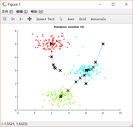
可以看到三堆点被很好地分成了三类。图片上同时也展示了中心点的移动轨迹。

1.3 Random initialization

ex7.m中为了方便检验结果正确性，给定了K的初始化。而实际应用中，我们需要随机初始化。
完成如下代码：

function centroids = kMeansInitCentroids(X, K)
%KMEANSINITCENTROIDS This function initializes K centroids that are to be 
%used in K-Means on the dataset X
%   centroids = KMEANSINITCENTROIDS(X, K) returns K initial centroids to be
%   used with the K-Means on the dataset X
%
% You should return this values correctly
centroids = zeros(K, size(X, 2));
% ====================== YOUR CODE HERE ======================
% Instructions: You should set centroids to randomly chosen examples from
%               the dataset X
%
% Initialize the centroids to be random examples
% Randomly reorder the indices of examples
randidx = randperm(size(X, 1));
% Take the first K examples as centroids
centroids = X(randidx(1:K), :);
% =============================================================
end

这样初始的中心点就是从X中随机选择的K个点。

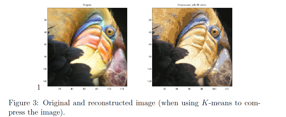
1.4 Image compression with K-means

用K-means进行图片压缩。
用一张$128\times 128$的图片为例，采用RGB，总共需要$128\times 128 \times 24 = 393216$个bit。
这里我们对他进行压缩，把所有颜色分成16类，以其centroid对应的颜色代替整个一类中的颜色，可以将空间压缩至$16\times 24 + 128\times 128 \times 4 = 65920$ 个bit。
用题目中提供的例子，效果大概如下：

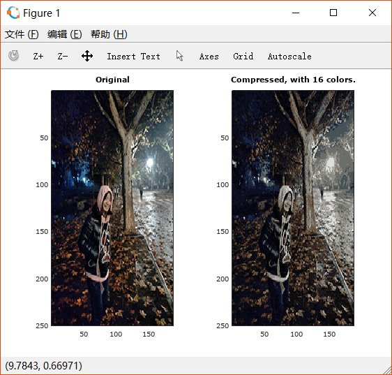
1.5 (Ungraded)Use your own image

随便找一张本地图片，先用PS调整大小，最好在 $256\times 256$ 以下（否则速度会很慢），运行，效果如下：

2 Principal component analysis

我们使用PCA来减少向量维数。

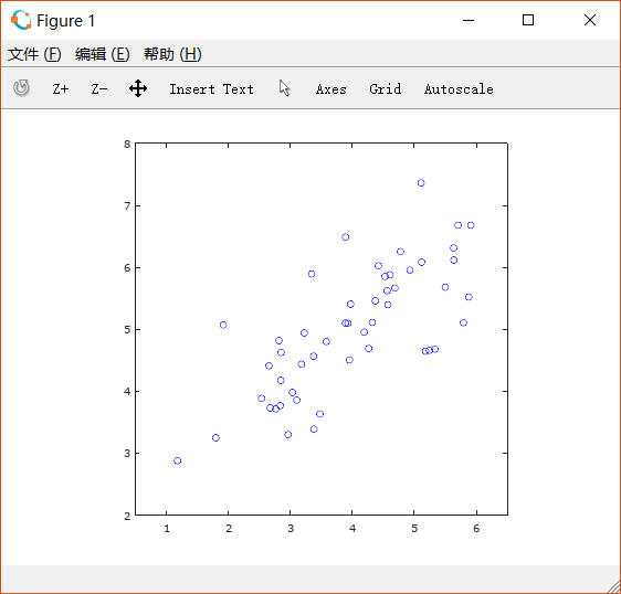
2.1 Example dataset

先对例子中的二维向量实现降低到一维。
绘制散点图如下：

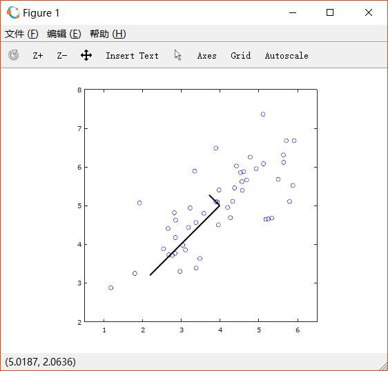
2.2 Implementing PCA

首先需要计算数据的协方差矩阵（covariance matrix）。
然后使用 Octave/MATLAB中的SVD函数计算特征向量（eigenvector）。

可以先对数据进行normalization和feature scaling的处理。
协方差矩阵如下计算：

然后用SVD函数求特征向量。
故完成pca.m如下：

function [U, S] = pca(X)
%PCA Run principal component analysis on the dataset X
%   [U, S, X] = pca(X) computes eigenvectors of the covariance matrix of X
%   Returns the eigenvectors U, the eigenvalues (on diagonal) in S
%
% Useful values
[m, n] = size(X);
% You need to return the following variables correctly.
U = zeros(n);
S = zeros(n);
% ====================== YOUR CODE HERE ======================
% Instructions: You should first compute the covariance matrix. Then, you
%               should use the "svd" function to compute the eigenvectors
%               and eigenvalues of the covariance matrix. 
%
% Note: When computing the covariance matrix, remember to divide by m (the
%       number of examples).
%
[U,S,V] = svd(1/m * X' * X);
% =========================================================================
end

把求出的特征向量绘制在图上：

2.3 Dimensionality reduction with PCA

将高维的examples投影到低维上。

2.3.1 Projecting the data onto the principal components

完成projectData.m如下：

function Z = projectData(X, U, K)
%PROJECTDATA Computes the reduced data representation when projecting only 
%on to the top k eigenvectors
%   Z = projectData(X, U, K) computes the projection of 
%   the normalized inputs X into the reduced dimensional space spanned by
%   the first K columns of U. It returns the projected examples in Z.
%
% You need to return the following variables correctly.
Z = zeros(size(X, 1), K);
% ====================== YOUR CODE HERE ======================
% Instructions: Compute the projection of the data using only the top K 
%               eigenvectors in U (first K columns). 
%               For the i-th example X(i,:), the projection on to the k-th 
%               eigenvector is given as follows:
%                    x = X(i, :)';
%                    projection_k = x' * U(:, k);
%
Ureduce = U(:,1:K);
Z = X * Ureduce;
% =============================================================
end

将X投影到K维空间上。

2.3.2 Reconstructing an approximation of the data

从投影过的低维恢复高维：

function X_rec = recoverData(Z, U, K)
%RECOVERDATA Recovers an approximation of the original data when using the 
%projected data
%   X_rec = RECOVERDATA(Z, U, K) recovers an approximation the 
%   original data that has been reduced to K dimensions. It returns the
%   approximate reconstruction in X_rec.
%
% You need to return the following variables correctly.
X_rec = zeros(size(Z, 1), size(U, 1));
% ====================== YOUR CODE HERE ======================
% Instructions: Compute the approximation of the data by projecting back
%               onto the original space using the top K eigenvectors in U.
%
%               For the i-th example Z(i,:), the (approximate)
%               recovered data for dimension j is given as follows:
%                    v = Z(i, :)';
%                    recovered_j = v' * U(j, 1:K)';
%
%               Notice that U(j, 1:K) is a row vector.
%               
Ureduce = U(:, 1:K);
X_rec = Z * Ureduce';
% =============================================================
end

2.3.3 Visualizing the projections

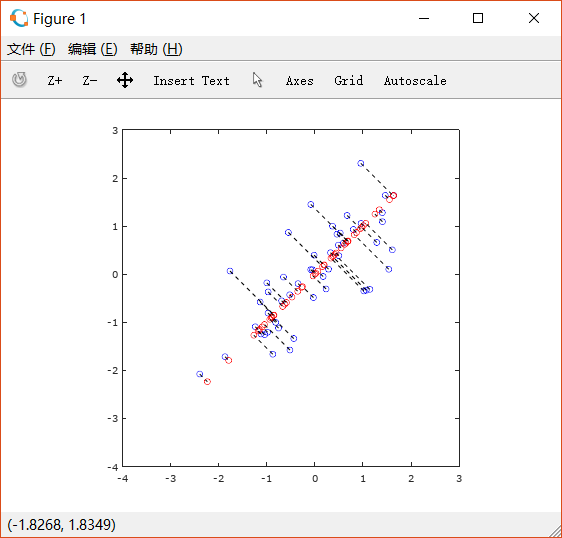
根据上图可以看出，恢复后的图只保留了其中一个特征向量上的信息，而垂直方向的信息丢失了。

2.4 Face image dataset

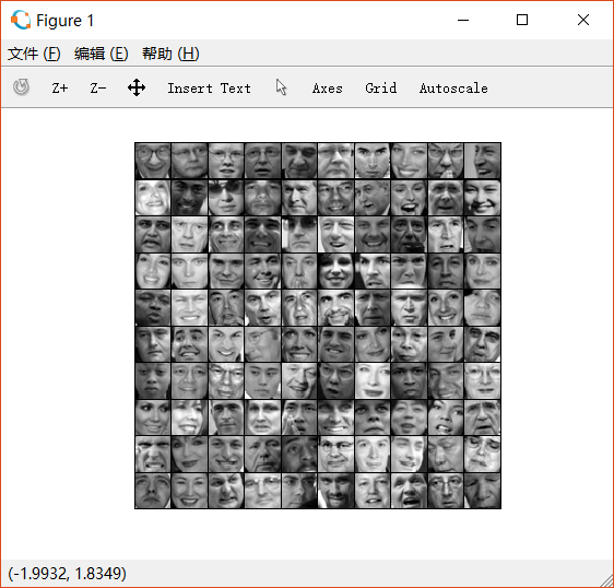
对人脸图片进行dimension reduction。ex7faces.mat中存有大量人脸的灰度图（$32 \times 32$) , 因此每一个向量的维数是 $32 \times 32 = 1024$。
如下是前一百张人脸图：

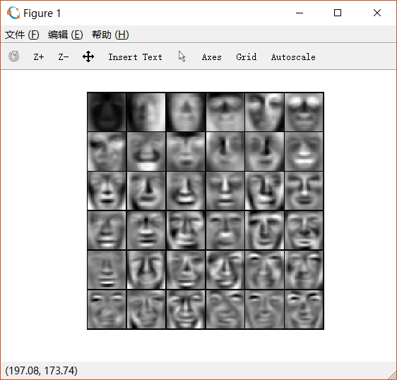
2.4.1 PCA on faces

用PCA得到其主成分，将其重新转化为 $32\times 32$ 的矩阵后，对其可视化，如下：(只展示前36个）

2.4.2 Dimensionality reduction

取前100个特征向量进行投影，

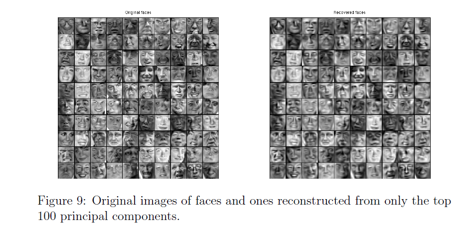
可以看出，降低维度后，人脸部的大致框架还保留着，但是失去了一些细节。这给我们的启发是，当我们在用神经网络训练人脸识别时，有时候可以用这种方式来提高速度。

2.5 Optional (Ungraded) exercise: PCA for visualization

PCA常用于高维向量的可视化。
如下图，用K-means对三维空间上的点进行分类。

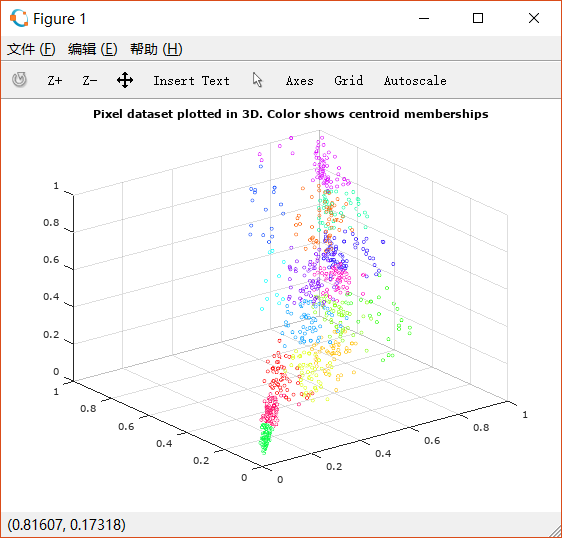
对图片进行旋转，可以看出这些点大致在一个平面上

因此我们使用PCA将其降低到二维，并观察散点图：

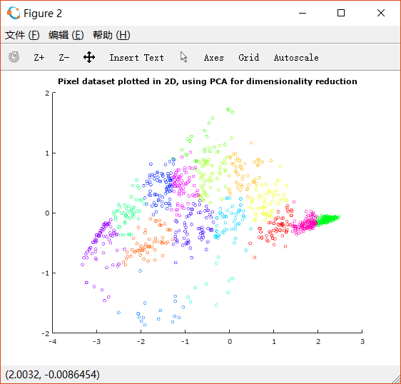
这样就更利于观察分类的情况了。