机器学习week6 ex5 review

吴恩达 机器学习

本周主要关于如何改进学习效果。

1 Regularized linear regression

1.1Plotting the data

绘制ex5data1.mat中关于水流量和坝中剩余水量的散点图。

%% =========== Part 1: Loading and Visualizing Data =============
%  We start the exercise by first loading and visualizing the dataset. 
%  The following code will load the dataset into your environment and plot
%  the data.
%
% Load Training Data
fprintf('Loading and Visualizing Data ...\n')
% Load from ex5data1: 
% You will have X, y, Xval, yval, Xtest, ytest in your environment
load ('ex5data1.mat');
% m = Number of examples
m = size(X, 1);
% Plot training data
plot(X, y, 'rx', 'MarkerSize', 10, 'LineWidth', 1.5);
xlabel('Change in water level (x)');
ylabel('Water flowing out of the dam (y)');
fprintf('Program paused. Press enter to continue.\n');
pause;

绘制情况如下：

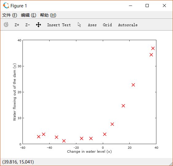
显然这个情况用直线拟合并不合适，我们先试着使用线性回归，之后再尝试更高次的多项式。

1.2 Regularized linear regression cost function

1.3 Regularized linear regression gradient

代价函数如下：

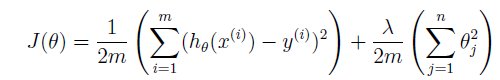
按照上述式子完成linearRegCostFunction.m：

function [J, grad] = linearRegCostFunction(X, y, theta, lambda)
%LINEARREGCOSTFUNCTION Compute cost and gradient for regularized linear 
%regression with multiple variables
%   [J, grad] = LINEARREGCOSTFUNCTION(X, y, theta, lambda) computes the 
%   cost of using theta as the parameter for linear regression to fit the 
%   data points in X and y. Returns the cost in J and the gradient in grad
% Initialize some useful values
m = length(y); % number of training examples
% You need to return the following variables correctly 
J = 0;
grad = zeros(size(theta));
% ====================== YOUR CODE HERE ======================
% Instructions: Compute the cost and gradient of regularized linear 
%               regression for a particular choice of theta.
%
%               You should set J to the cost and grad to the gradient.
%
htheta = X * theta;
J = 1 / (2 * m) * sum((htheta - y) .^ 2) + lambda / (2 * m) * sum(theta(2:end) .^ 2);
grad = 1 / m * X' * (htheta - y);
grad(2:end) = grad(2:end) + lambda / m * theta(2:end);
% =========================================================================
grad = grad(:);
end

结果正确，不消多提。

1.4 Fitting linear regression

trainlinearReg.m中利用fimincg函数实现线性回归：

function [theta] = trainLinearReg(X, y, lambda)
%TRAINLINEARREG Trains linear regression given a dataset (X, y) and a
%regularization parameter lambda
%   [theta] = TRAINLINEARREG (X, y, lambda) trains linear regression using
%   the dataset (X, y) and regularization parameter lambda. Returns the
%   trained parameters theta.
%
% Initialize Theta
initial_theta = zeros(size(X, 2), 1); 
% Create "short hand" for the cost function to be minimized
costFunction = @(t) linearRegCostFunction(X, y, t, lambda);
% Now, costFunction is a function that takes in only one argument
options = optimset('MaxIter', 200, 'GradObj', 'on');
% Minimize using fmincg
theta = fmincg(costFunction, initial_theta, options);
end

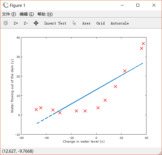
ex5.m用训练出来的 $\theta$ 做图：

%  Train linear regression with lambda = 0
lambda = 0;
[theta] = trainLinearReg([ones(m, 1) X], y, lambda);
%  Plot fit over the data
plot(X, y, 'rx', 'MarkerSize', 10, 'LineWidth', 1.5);
xlabel('Change in water level (x)');
ylabel('Water flowing out of the dam (y)');
hold on;
plot(X, [ones(m, 1) X]*theta, '--', 'LineWidth', 2)
hold off;
fprintf('Program paused. Press enter to continue.\n');
pause;

2 Bias variance

high bias: underfitting
high variance: overfitting

2.1 Learning curves

将training example划分为training set和cross validation set
training error:

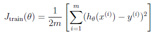
可用现有的cost function的函数将lambda设置为0直接计算。
代码如下：

function [error_train, error_val] = ...
    learningCurve(X, y, Xval, yval, lambda)
%LEARNINGCURVE Generates the train and cross validation set errors needed 
%to plot a learning curve
%   [error_train, error_val] = ...
%       LEARNINGCURVE(X, y, Xval, yval, lambda) returns the train and
%       cross validation set errors for a learning curve. In particular, 
%       it returns two vectors of the same length - error_train and 
%       error_val. Then, error_train(i) contains the training error for
%       i examples (and similarly for error_val(i)).
%
%   In this function, you will compute the train and test errors for
%   dataset sizes from 1 up to m. In practice, when working with larger
%   datasets, you might want to do this in larger intervals.
%
% Number of training examples
m = size(X, 1);
% You need to return these values correctly
error_train = zeros(m, 1);
error_val   = zeros(m, 1);
% ====================== YOUR CODE HERE ======================
% Instructions: Fill in this function to return training errors in 
%               error_train and the cross validation errors in error_val. 
%               i.e., error_train(i) and 
%               error_val(i) should give you the errors
%               obtained after training on i examples.
%
% Note: You should evaluate the training error on the first i training
%       examples (i.e., X(1:i, :) and y(1:i)).
%
%       For the cross-validation error, you should instead evaluate on
%       the _entire_ cross validation set (Xval and yval).
%
% Note: If you are using your cost function (linearRegCostFunction)
%       to compute the training and cross validation error, you should 
%       call the function with the lambda argument set to 0. 
%       Do note that you will still need to use lambda when running
%       the training to obtain the theta parameters.
%
% Hint: You can loop over the examples with the following:
%
%       for i = 1:mx
%           % Compute train/cross validation errors using training examples 
%           % X(1:i, :) and y(1:i), storing the result in 
%           % error_train(i) and error_val(i)
%           ....
%           
%       end
%
% ---------------------- Sample Solution ----------------------
for i = 1:m,
  theta = trainLinearReg(X(1:i,:),y(1:i),lambda);
  error_train(i) = linearRegCostFunction(X(1:i,:),y(1:i),theta,0);
  error_val(i) = linearRegCostFunction(Xval,yval,theta,0);
end;
% -------------------------------------------------------------
% =========================================================================
end

脚本文件中这部分:

%% =========== Part 5: Learning Curve for Linear Regression =============
%  Next, you should implement the learningCurve function. 
%
%  Write Up Note: Since the model is underfitting the data, we expect to
%                 see a graph with "high bias" -- Figure 3 in ex5.pdf 
%
lambda = 0;
[error_train, error_val] = ...
    learningCurve([ones(m, 1) X], y, ...
                  [ones(size(Xval, 1), 1) Xval], yval, ...
                  lambda);
plot(1:m, error_train, 1:m, error_val);
title('Learning curve for linear regression')
legend('Train', 'Cross Validation')
xlabel('Number of training examples')
ylabel('Error')
axis([0 13 0 150])
fprintf('# Training Examples\tTrain Error\tCross Validation Error\n');
for i = 1:m
    fprintf('  \t%d\t\t%f\t%f\n', i, error_train(i), error_val(i));
end
fprintf('Program paused. Press enter to continue.\n');
pause;

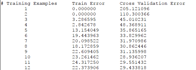
绘制的图像如下：

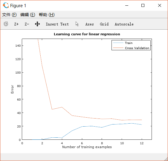
这显然是underfitting的情况，即high bias，在这种情况下继续增加training examples几乎没有效果。

3 Polynomial regression

刚才的实验证明简单的线性回归无法很好地拟合情况，因此我们采用多项式回归。

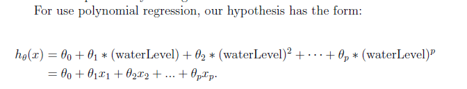
令$x_1 = waterlevel, x_2 = (waterlevel)^2...x_p = (waterlevel)^p$ 可以将其转化为多元的线性回归。
因此将X改写成X_poly：

unction [X_poly] = polyFeatures(X, p)
%POLYFEATURES Maps X (1D vector) into the p-th power
%   [X_poly] = POLYFEATURES(X, p) takes a data matrix X (size m x 1) and
%   maps each example into its polynomial features where
%   X_poly(i, :) = [X(i) X(i).^2 X(i).^3 ...  X(i).^p];
%
% You need to return the following variables correctly.
X_poly = zeros(numel(X), p);
% ====================== YOUR CODE HERE ======================
% Instructions: Given a vector X, return a matrix X_poly where the p-th 
%               column of X contains the values of X to the p-th power.
%
% 
for i = 1:p,
  X_poly(:,i) = X.^2;
end;
% =========================================================================
end

3.1 Learning polynomial regression

进行完这步之后需要进行Normalization的操作。这个在ex1中已经实现过了。此处不表。

脚本文件执行learning polynomial regression的部分（已经完成了Normalization）：

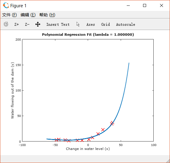
%% =========== Part 7: Learning Curve for Polynomial Regression =============
%  Now, you will get to experiment with polynomial regression with multiple
%  values of lambda. The code below runs polynomial regression with 
%  lambda = 0. You should try running the code with different values of
%  lambda to see how the fit and learning curve change.
%
lambda = 0;
[theta] = trainLinearReg(X_poly, y, lambda);
% Plot training data and fit
figure(1);
plot(X, y, 'rx', 'MarkerSize', 10, 'LineWidth', 1.5);
plotFit(min(X), max(X), mu, sigma, theta, p);
xlabel('Change in water level (x)');
ylabel('Water flowing out of the dam (y)');
title (sprintf('Polynomial Regression Fit (lambda = %f)', lambda));
figure(2);
[error_train, error_val] = ...
    learningCurve(X_poly, y, X_poly_val, yval, lambda);
plot(1:m, error_train, 1:m, error_val);
title(sprintf('Polynomial Regression Learning Curve (lambda = %f)', lambda));
xlabel('Number of training examples')
ylabel('Error')
axis([0 13 0 100])
legend('Train', 'Cross Validation')
fprintf('Polynomial Regression (lambda = %f)\n\n', lambda);
fprintf('# Training Examples\tTrain Error\tCross Validation Error\n');
for i = 1:m
    fprintf('  \t%d\t\t%f\t%f\n', i, error_train(i), error_val(i));
end
fprintf('Program paused. Press enter to continue.\n');
pause;

绘制如下两图：


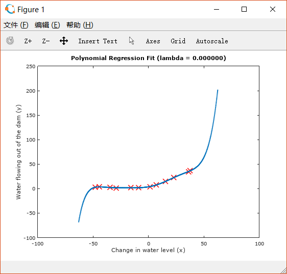
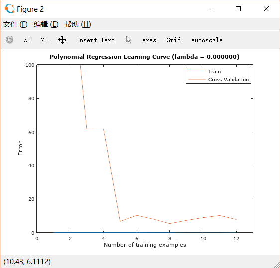
从第一张图可以看出，执行的回归对training set中的点拟合得非常好。但图像形状过于复杂，在两端极限处斜率很大，很可能发生了overfitting。
图二的training error印证了这一点，无论training example的数量如何增加，training error始终为0, 而cross validation error起初非常大，随着training set的增加，在逐渐变小。这说明，当前的状况属于overfitting。
在之前的学习中我们知道，引入regularization可以解决overfit的问题。

3.2 Adjust the regularization parameter

修改脚本文件中lambda的取值，观察图形变化。

• 设置lambda=1：
  
  
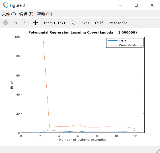
  可以看出此时拟合得很好，而且从learning curve来看，它既不是high bias也不是high variance, 而是实现了一个很好的bias-variance tradeoff。

• 设置lambda=100:
  
  
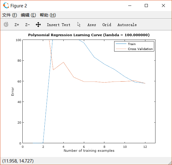
  很明显，由于lambda的值设置得过大，导致出现了underfit的问题。
  此时的问题是high bias。

3.3 selecting lambda using a validation set

对一组lambda分别计算其train error和cross validation error，绘制图像，以选择最合适的lambda。如下代码，将计算结果分别存入error_train和lambda_val中：

function [lambda_vec, error_train, error_val] = ...
    validationCurve(X, y, Xval, yval)
%VALIDATIONCURVE Generate the train and validation errors needed to
%plot a validation curve that we can use to select lambda
%   [lambda_vec, error_train, error_val] = ...
%       VALIDATIONCURVE(X, y, Xval, yval) returns the train
%       and validation errors (in error_train, error_val)
%       for different values of lambda. You are given the training set (X,
%       y) and validation set (Xval, yval).
%
% Selected values of lambda (you should not change this)
lambda_vec = [0 0.001 0.003 0.01 0.03 0.1 0.3 1 3 10]';
% You need to return these variables correctly.
error_train = zeros(length(lambda_vec), 1);
error_val = zeros(length(lambda_vec), 1);
% ====================== YOUR CODE HERE ======================
% Instructions: Fill in this function to return training errors in 
%               error_train and the validation errors in error_val. The 
%               vector lambda_vec contains the different lambda parameters 
%               to use for each calculation of the errors, i.e, 
%               error_train(i), and error_val(i) should give 
%               you the errors obtained after training with 
%               lambda = lambda_vec(i)
%
% Note: You can loop over lambda_vec with the following:
%
%       for i = 1:length(lambda_vec)
%           lambda = lambda_vec(i);
%           % Compute train / val errors when training linear 
%           % regression with regularization parameter lambda
%           % You should store the result in error_train(i)
%           % and error_val(i)
%           ....
%           
%       end
%
%
for i = 1:length(lambda_vec)
  lambda = lambda_vec(i);
  theta = trainLinearReg(X,y,lambda);
  error_train(i) = linearRegCostFunction(X, y, theta, 0);
  error_val(i) = linearRegCostFunction(Xval, yval, theta, 0);
end;
% =========================================================================
end

脚本文件执行作图操作：

%% =========== Part 8: Validation for Selecting Lambda =============
%  You will now implement validationCurve to test various values of 
%  lambda on a validation set. You will then use this to select the
%  "best" lambda value.
%
[lambda_vec, error_train, error_val] = ...
    validationCurve(X_poly, y, X_poly_val, yval);
close all;
plot(lambda_vec, error_train, lambda_vec, error_val);
legend('Train', 'Cross Validation');
xlabel('lambda');
ylabel('Error');
fprintf('lambda\t\tTrain Error\tValidation Error\n');
for i = 1:length(lambda_vec)
    fprintf(' %f\t%f\t%f\n', ...
            lambda_vec(i), error_train(i), error_val(i));
end
fprintf('Program paused. Press enter to continue.\n');
pause;

绘制图形如下：

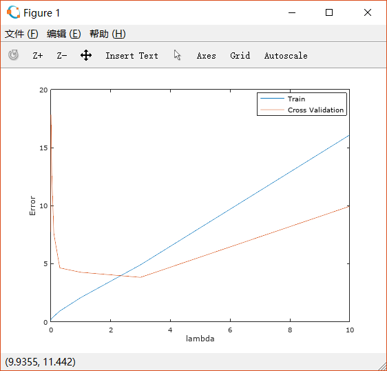
根据cross validation error的图像，可以看出最佳的lambda取值应该大致在3左右的范围内。

3.4 Computing test error

经过training和cross validation的过程后，我们得到了最合适的 $\theta$ 和 $\lambda$ ， 但一般来说，我们还需要对一些之前没有使用过的数据进行test，并计算test error。

3.5 Plotting learning curves with randomly selected examples

在绘制learning curve的时候，我们选取的增加training example 的方式是按顺序逐渐增加，而更好的做法应该是对第i个循环，随机选取i个training example来得到theta，并用这个theta来计算对应的train error和cross validation error。