Exercise 12

problem 5.7:The jacobi method v.s. The SOR algorithm

Problem 5.7
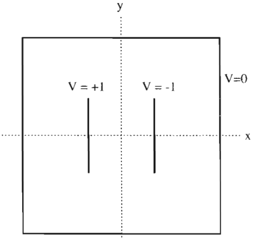
$\qquad$ Write two programs to solve the capacitor problem of Figure 5.6 and 5.7, one using Jacobi method and one using simultaneous over relaxation (SOR) algrithem . For a fixed accuracy (as set by the convergence test) compare the number of iterations,$N_{iter}$, that each algrithm requires as a function of the number of grid elements, L. Show that for Jacobi method $N_{iter}$~$L^2$, while with SOR $N_{iter}$~$L$ .

Abstract

$\qquad$ The partial differential equation is of physicists' great interest for its widely applicaiton in decribing physical systems. Jacobi method and simultaneous over relaxation (SOR) method are two algrithm that keep a balance of the simplicity for comprehension and accuracy of computation. This article made a comparsion between Jacobi method and SOR algorithm to solve partial differential equation. Also, it compared the number of iterations and figured out the relation between the number of iterations and the number of grid elements.

Background

Introduction

$\qquad$As we known, the electric potential satisfies Laplace's equation in the space without any electric charges.

$$▽^2V=\frac{∂^2V}{∂x^2}+\frac{∂^2V}{∂y^2}+\frac{∂^2V}{∂z^2}=0$$
$\qquad$After some calculation,we find
$$V(i,j,k)=\frac{1}{6}[V(i+1,j,k)+V(i-1,j,k)+V(i,j+1,k)$$
$$+V(i,j-1,k) +V(i,j,k+1)+V(i,j,k-1)]$$
$\qquad$AsSpecially, for the 2-dimensional case:
$$V(i,j,k)=\frac{1}{4}[V(i+1,j,k)+V(i-1,j,k)+V(i,j+1,k)+V(i,j-1,k)]$$

● Jacobi Method

$\qquad$ In numerical linear algebra, the Jacobi method (or Jacobi iterative method) is an algorithm for determining the solutions of a diagonally dominant system of linear equations. Each diagonal element is solved for, and an approximate value is plugged in. The process is then iterated until it converges. This algorithm is a stripped-down version of the Jacobi transformation method of matrix diagonalization. The method is named after Carl Gustav Jacob Jacobi.
$\qquad$ If we only use the old potential to calculate the new one, the formula becomes:

$$V_{new}(i,j,k)=\frac{1}{4}[V_{old}(i+1,j,k)+V_{old}(i-1,j,k)+V_{old}(i,j+1,k)+V_{old}(i,j-1,k)]$$ $\qquad$ This is what we called Jacobi method.

● Simultaneous Over Relaxation (SOR) Method

$\qquad$ In numerical linear algebra, the method of successive over-relaxation (SOR) is a variant of the Gauss–Seidel method for solving a linear system of equations, resulting in faster convergence. A similar method can be used for any slowly converging iterative process.
$\qquad$ Obviously, we can make use of the new values as they become available, which means:

$$V^*(i,j,k)=\frac{1}{4}[V_{old}(i+1,j,k)+V_{new}(i-1,j,k)+V_{old}(i,j+1,k)+V_{new}(i,j-1,k)]$$ $\qquad$ We can then think of
$$△V(i,j)≡V^*(i,j)-V_{old}(i,j)$$ $\qquad$ as the change recommend by the Gauss-Seidel algorithm. However, this choice $△V(i,j)$ is too conservative. So to speed up convergence we will change he potential by a larger amount calculated according to
$$V_{new}(i,j)=V_{old}(i,j)+α△V(i,j)$$ $\qquad$ This is what we called SOR algorithm. Generally, we set $α=\frac{2}{1+π/L}$ for the Dirichlet boundary conditions.

$\qquad$ It was devised simultaneously by David M. Young, Jr. and by H. Frankel in 1950 for the purpose of automatically solving linear systems on digital computers. Over-relaxation methods had been used before the work of Young and Frankel. An example is the method of Lewis Fry Richardson, and the methods developed by R. V. Southwell. However, these methods were designed for computation by human calculators, and they required some expertise to ensure convergence to the solution which made them inapplicable for programming on digital computers. These aspects are discussed in the thesis of David M. Young, Jr.

main body

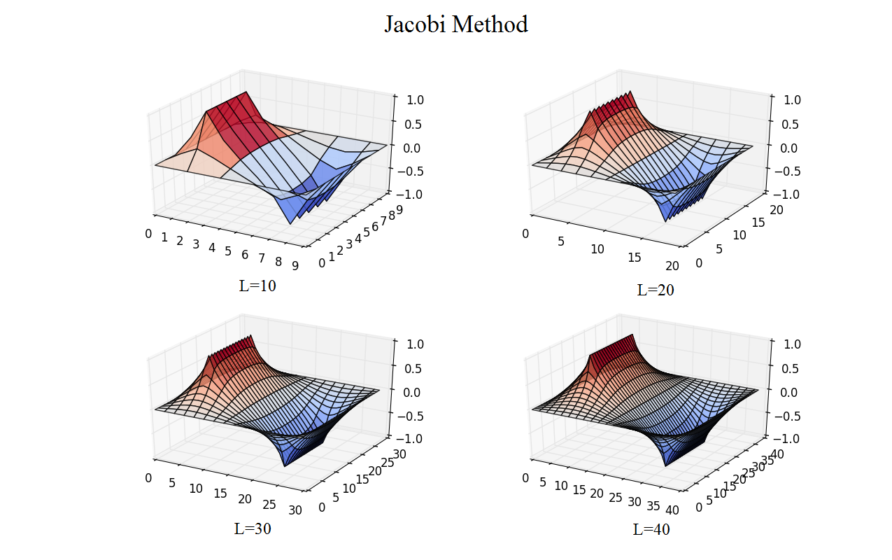
Figure 12.1 Fitting curve of interating time versus time step; the expresssion is given in the figure.

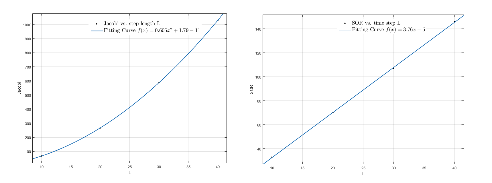
Figure 13.2 Fitting curve of interating time versus time step; the expresssion is given in the figure.

Step Length	Jacobi Method	SOR method
10	68	8.536
20	265	70
30	589	107
40	1028	146

Jacobi method

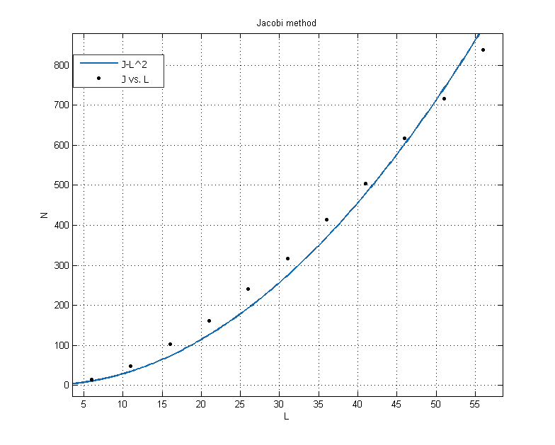
Fit equation:$N=a*L^2$
$a=0.2894$
$R^2=0.9834$
The number of iterations N is about proportional to $L^2$

SOR method

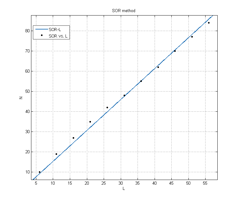
Fit equation:$N=a*L^2$
$a=1.531$
$R^2=0.9949$
The number of iterations N is approximately proportional to L.

The fitting results are $0.2772L^2$ for the blue curve and $1.701L$ for the red one, which means the number of iteration is proportional to $L^2$ for jacobi method and is proportional to L for SOR algorithm.Therefore, the larger grid we used, the bigger advantage of SOR algorithm would be showed.

The Convergence speed

On the other hand, we can make a comparison of the convergence speed of these methods.

The convergence speed of SOR algorithm is much larger than that of jacobi method.

The α of SOR algorithm

Additionally, I make a discussion of the relation between the number of iteration and the value of α.

In this case, I set the length of grid is 26, which means the value of α is about 1.784. Obviously, this is α not the best choice to decrease the number of iterations.

Conclusion

● I solved the electric potential and field of exercise 5.7.
● Comparing 2 different methods, the convergent speeds:SOR method > Jacobi method.
● At the same accuracy, using Jacobi method, the number of iterations N is about proportional to $L^2$;while using SOR method, the number of iterations N is about proportional to $L$.

Reference

1. Giodano, N.J., Nakanishi, H. Computational Physics. Tsinghua University Press, December 2007
2. Jacobi method. (2016, May 16). In Wikipedia, The Free Encyclopedia. Retrieved 12:47, May 22, 2016, from https://en.wikipedia.org/w/index.php?title=Jacobi_method&oldid=720500900
3. Successive over-relaxation. (2016, April 27). In Wikipedia, The Free Encyclopedia. Retrieved 12:46, May 22, 2016, from https://en.wikipedia.org/w/index.php?title=Successive_over-relaxation&oldid=717363228
4. Thanks to Chen Feng and Wang Shixing

Codes