@lumincinta
2017-02-07T12:31:13.000000Z
字数 5523
阅读 315
R Package 'smbinning' V0.3: Optimal Binning for Scoring Modeling
R.Package
Reference
Scoring Modeling - Data, Analysis, and Scoring Modeling
Description
The package smbinning categorizes a numeric variable into bins or bands mapped to a binary target variable for its ulterior usage in scoring modeling. Its purpose is to automate the time consuming process of selecting the right cut points, quickly calculate metrics such as Weight of Evidence and Information Value (IV); and also document SQL codes, tables, and plots used throughout the development stage.
In its new Version 0.3, the package allows the user in one step (smbinning.eda) to see missing values and outliers for each characteristic in the dataset, along with basic statistics to better understand their distribution, and also in one step obtain the Information Value for each characteristic (smbinning.sumiv).
The desired outputs are basically the tables showed in the examples below, whose theory can be found in the following books:
- "Credit Scoring, Response Modeling, and Insurance Rating" (Finlay, 2010). See it [Here]
- "The Credit Scoring Toolkit" (Anderson, 2007). See it [Here]
- "Credit Risk Scorecards" (Siddiqi, 2006). See it [Here]
More details on:
What's New on Version 0.3?
- New function that calculates IV for all variables in one step.
- New function that plots and ranks IVs for each variable.
- New function for exploratory data analysis.
- New function that produces SQL code after binning factors.
- New function that generate variables after binning factors.
- Variables generated after binning now are factors with labels, instead of character.
- Modified dataset that allows a better understanding of the new functionalities.
# ----------------------------------------------------# Package : Optimal Binning for Scoring Modeling V0.3# Author : Herman Jopia# Website : http://www.scoringmodeling.com# Twitter : @hjopia# ----------------------------------------------------# Load package and its datalibrary(smbinning)data(chileancredit)str(chileancredit) # Quick description of the datatable(chileancredit$FlagGB) # Tabulate target variabletable(chileancredit$FlagSample) # 2 random samples (1:75%, 0:25%)# Training and testing sampleschileancredit.train=subset(chileancredit,FlagSample==1)chileancredit.test=subset(chileancredit,FlagSample==0)# Optimal Binning ----------------------------------------------------------result=smbinning(df=chileancredit.train,y="FlagGB",x="TOB",p=0.05) # Run and saveresult$ivtable # Tabulation and Information Valueresult$iv # Information valueresult$bands # Bins or bandsresult$ctree # Decision tree from partykit# Relevant plots (2x2 Page)par(mfrow=c(2,2))boxplot(chileancredit.train$TOB~chileancredit.train$FlagGB,horizontal=T, frame=F, col="lightgray",main="Distribution")mtext("Time on Books (Months)",3)smbinning.plot(result,option="dist",sub="Time on Books (Months)")smbinning.plot(result,option="badrate",sub="Time on Books (Months)")smbinning.plot(result,option="WoE",sub="Time on Books (Months)")# SQL Code after binning a numeric variable ---------------------------------smbinning.sql(result)# Generate variable after binning -------------------------------------------chileancredit=smbinning.gen(chileancredit, result, chrname = "gTOB")# Customized Binning --------------------------------------------------------# Remove exclusions from chileancredit datasetTOB.train=subset(chileancredit,(FlagSample==1 & (FlagGB==1 | FlagGB==0)), select=TOB)# Percentiles of 20%TOB.Pct20=quantile(TOB.train, probs=seq(0,1,0.2), na.rm=T)TOB.Pct20.Breaks=as.vector(quantile(TOB.train, probs=seq(0,1,0.2), na.rm=T))Cuts.TOB.Pct20=TOB.Pct20.Breaks[2:(length(TOB.Pct20.Breaks)-1)]# Package application and resultsresult=smbinning.custom(df=chileancredit.train,y="FlagGB",x="TOB",cuts=Cuts.TOB.Pct20) # Run and saveresult$ivtable # Tabulation and Information Value# Factor Variable Application -----------------------------------------------result=smbinning.factor(df=chileancredit.train,y="FlagGB",x="IncomeLevel")result$ivtable# SQL Code after binning a factor variable ----------------------------------smbinning.sql(result)# Generate variable after binning factor ------------------------------------chileancredit=smbinning.factor.gen(chileancredit, result, chrname = "gInc")# Exploratory Data Analysis -------------------------------------------------smbinning.eda(df=chileancredit.train)$eda # Table with basic statisticssmbinning.eda(df=chileancredit.train)$edapct # Table with basic percentages# Information Value for all variables in one step ---------------------------smbinning.sumiv(df=chileancredit.train,y="FlagGB") # IV for eache variable# Plot IV for all variables -------------------------------------------------sumivt=smbinning.sumiv(chileancredit.train,y="FlagGB")sumivt # Display table with IV by characteristicpar(mfrow=c(1,1))smbinning.sumiv.plot(sumivt,cex=1) # Plot IV summary table
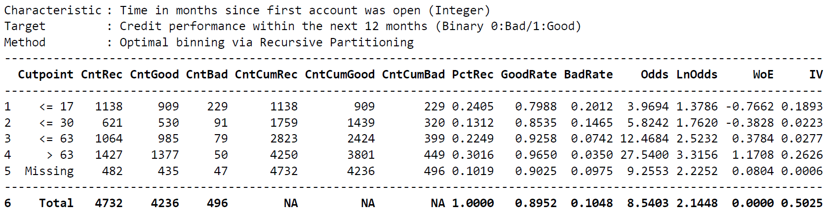
Table 1. Time on Books and Credit Performance via Optimal Binning. Plots from this output are shown in Figure 1 (Below).
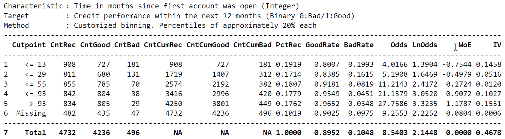
Table 2. Time on Books and Credit Performance utilizing customized cutpoints.
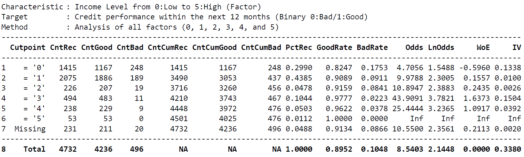
Table 3. Income Levels and Credit Performance. The package allows users to take advantage of its functionalities to analyze factor variables.

Figure 1. Time on Books and Credit Performance plots after Optimal Binning (Table 1).
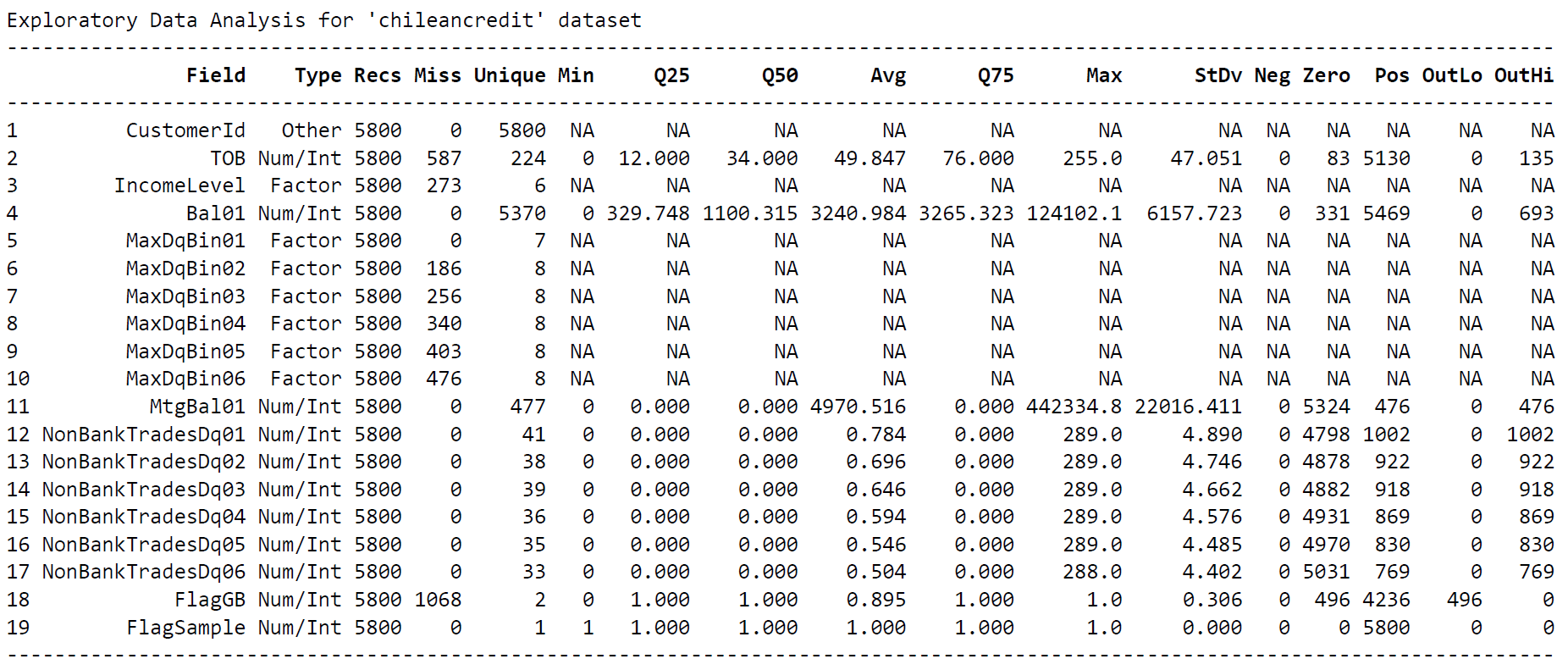
Table 4. Basic statistics to better understand each variable.
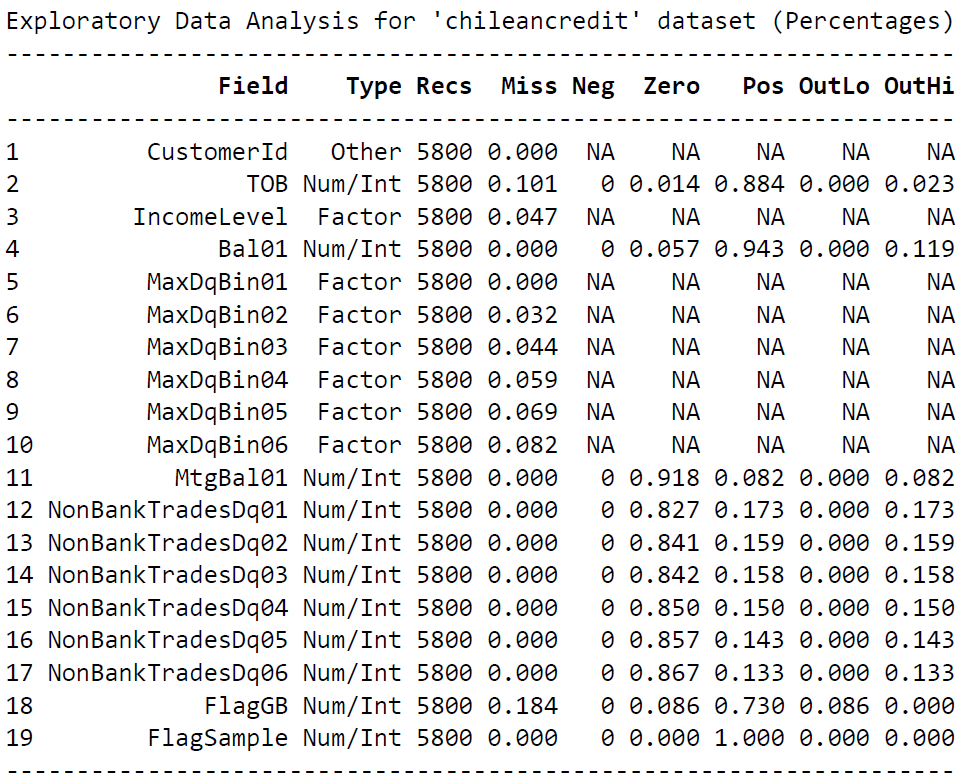
Table 5. Basic percentages that gives a different perspective of the numbers.
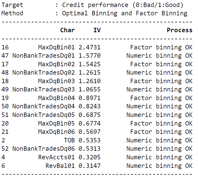
Table 6. IV for each characteristic of the dataset.
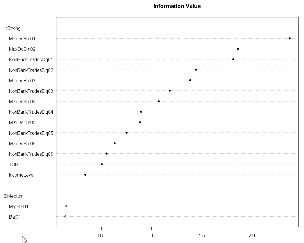
Figure 2. Plot the IV for each characteristic of the dataset.
Package History
- 2016-06-21: Version 0.3 available on CRAN (Happy!)
- 2015-06-15: Version 0.2 available on CRAN (Awesome!)
- 2015-03-24: Package featured on RevolutionAnalytics [Here]
- 2015-02-22: Package featured on Data Science Central [Here]
- 2015-02-16: Version 0.1 available as Binary Package, meaning,
install.packages("smbinning")can be used to install it. - 2015-02-15: Version 0.1 available on CRAN as a Source Package (Great!)
- 2014-10-19: Inception while writing about binning using recursive partitioning.
