@HaomingJiang 2018-03-01T04:12:26.000000Z 字数 23568 阅读 1547

HW 3

Haoming Jiang

Ex 3.1

a

3.1.1.png-3.4kB

> #########################################################################
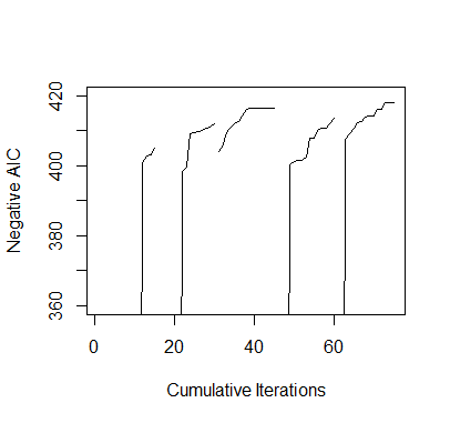
> ### EXERCISE 3.1
> #########################################################################
> # baseball.dat    = entire data set
> # baseball.sub    = matrix of all predictors
> # salary.log  = response, log salary
> # n       = number of observations in the data set
> # m       = number of predictors in the data set
> # num.starts  = number of random starts
> # runs        = matrix containing the random starts where each row is a
> #           vector of the parameters included for the model
> #           (1 = included, 0 = omitted)
> # runs.aic    = AIC values for the best model found for each
> #           of the random starts
> # itr         = number of iterations for each random start
> #########################################################################
> 
> ## INITIAL VALUES
> baseball.dat = read.table("baseball.dat",header=TRUE)
> baseball.dat$freeagent = factor(baseball.dat$freeagent)
> baseball.dat$arbitration = factor(baseball.dat$arbitration)
> baseball.sub = baseball.dat[,-1]
> salary.log = log(baseball.dat$salary)
> n = length(salary.log)
> m = length(baseball.sub[1,])
> num.starts = 5
> runs = matrix(0,num.starts,m)
> itr = 15
> runs.aic = matrix(0,num.starts,itr)
> 
> # INITIALIZES STARTING RUNS
> set.seed(19676) 
> for(i in 1:num.starts){runs[i,] = rbinom(m,1,.5)}
> 
> ## MAIN
> for(k in 1:num.starts){
+   run.current = runs[k,]
+   
+   # ITERATES EACH RANDOM START
+   for(j in 1:itr){
+     run.vars = baseball.sub[,run.current==1]
+     g = lm(salary.log~.,run.vars)
+     run.aic = extractAIC(g)[2]
+     run.next = run.current
+     
+     # TESTS ALL MODELS IN THE 1-NEIGHBORHOOD AND SELECTS THE
+     # MODEL WITH THE LOWEST AIC
+     for(i in sample(m)){
+       run.step = run.current
+       run.step[i] = !run.current[i]
+       run.vars = baseball.sub[,run.step==1]
+       g = lm(salary.log~.,run.vars)
+       run.step.aic = extractAIC(g)[2]
+       if(run.step.aic < run.aic){
+         run.next = run.step
+         run.aic = run.step.aic
+         break
+       }
+     }
+     run.current = run.next
+     runs.aic[k,j]=run.aic
+   }
+   runs[k,] = run.current
+ }
> 
> ## OUTPUT
> runs      # LISTS OF PREDICTORS
     [,1] [,2] [,3] [,4] [,5] [,6] [,7] [,8] [,9] [,10] [,11] [,12] [,13] [,14] [,15] [,16]
[1,]    1    0    0    1    0    0    1    0    1     1     0     0     1     1     1     0
[2,]    1    0    1    0    0    1    0    1    0     1     1     0     1     1     1     1
[3,]    0    0    1    0    0    1    0    1    0     1     0     0     1     1     1     0
[4,]    1    1    1    0    0    1    0    1    0     1     0     0     1     1     1     1
[5,]    1    0    1    0    0    0    0    1    0     1     0     0     1     1     1     1
     [,17] [,18] [,19] [,20] [,21] [,22] [,23] [,24] [,25] [,26] [,27]
[1,]     0     1     1     0     0     0     0     0     1     0     1
[2,]     1     1     0     0     1     0     0     1     0     1     1
[3,]     0     0     0     1     1     1     0     0     1     1     0
[4,]     0     0     0     0     0     1     1     1     1     1     0
[5,]     0     0     0     0     0     0     0     1     1     0     1
> runs.aic  # AIC VALUES
          [,1]      [,2]      [,3]      [,4]      [,5]      [,6]      [,7]      [,8]
[1,] -217.9065 -217.9935 -219.8484 -220.1619 -221.0135 -222.6077 -223.7776 -223.9698
[2,] -217.2085 -218.3258 -219.5092 -219.7432 -221.7374 -223.6676 -398.4278 -399.6693
[3,] -403.9695 -405.3088 -409.3507 -410.7968 -411.9632 -412.6045 -414.2432 -416.2141
[4,] -124.5394 -127.0578 -127.5083 -400.2682 -401.1612 -401.6403 -401.6661 -402.5395
[5,] -135.9155 -137.7239 -407.5777 -409.1986 -410.8303 -412.4298 -412.6726 -413.9250
          [,9]     [,10]     [,11]     [,12]     [,13]     [,14]     [,15]
[1,] -225.8663 -232.0466 -233.5325 -400.9725 -402.8854 -403.2838 -404.8729
[2,] -409.1566 -409.3218 -409.6924 -410.1146 -410.6694 -411.0543 -412.0218
[3,] -416.5069 -416.5069 -416.5069 -416.5069 -416.5069 -416.5069 -416.5069
[4,] -407.9254 -407.9608 -410.2451 -410.6919 -410.8825 -411.9445 -413.5147
[5,] -414.0846 -414.2130 -416.1533 -416.2576 -417.8858 -417.8858 -417.8858
> 
> ##PLOT
> plot(1:(itr*num.starts),-c(t(runs.aic)),xlab="Cumulative Iterations",
+      ylab="Negative AIC",ylim=c(360,420),type="n")
> for(i in 1:num.starts) {
+   lines((i-1)*itr+(1:itr),-runs.aic[i,]) }

b

It takes longer time. And AIC are much greater than the previouse ones. All because somtimes it can not find a downhill 2-neighborhood.
3.1.2.png-2.9kB

> #########################################################################
> ### EXERCISE 3.1
> #########################################################################
> # baseball.dat    = entire data set
> # baseball.sub    = matrix of all predictors
> # salary.log  = response, log salary
> # n       = number of observations in the data set
> # m       = number of predictors in the data set
> # num.starts  = number of random starts
> # runs        = matrix containing the random starts where each row is a
> #           vector of the parameters included for the model
> #           (1 = included, 0 = omitted)
> # runs.aic    = AIC values for the best model found for each
> #           of the random starts
> # itr         = number of iterations for each random start
> #########################################################################
> 
> ## INITIAL VALUES
> baseball.dat = read.table("baseball.dat",header=TRUE)
> baseball.dat$freeagent = factor(baseball.dat$freeagent)
> baseball.dat$arbitration = factor(baseball.dat$arbitration)
> baseball.sub = baseball.dat[,-1]
> salary.log = log(baseball.dat$salary)
> n = length(salary.log)
> m = length(baseball.sub[1,])
> num.starts = 5
> runs = matrix(0,num.starts,m)
> itr = 15
> runs.aic = matrix(0,num.starts,itr)
> 
> # INITIALIZES STARTING RUNS
> set.seed(19676) 
> for(i in 1:num.starts){runs[i,] = rbinom(m,1,.5)}
> 
> all2combn = combn(m,2)
> 
> ## MAIN
> for(k in 1:num.starts){
+   run.current = runs[k,]
+   
+   # ITERATES EACH RANDOM START
+   for(j in 1:itr){
+     run.vars = baseball.sub[,run.current==1]
+     g = lm(salary.log~.,run.vars)
+     run.aic = extractAIC(g)[2]
+     run.next = run.current
+     
+     # TESTS ALL MODELS IN THE 1-NEIGHBORHOOD AND SELECTS THE
+     # MODEL WITH THE LOWEST AIC
+     for(i in sample(m*(m-1)/2)){
+       run.step = run.current
+       run.step[all2combn[1][i]] = !run.current[all2combn[1][i]]
+       run.step[all2combn[2][i]] = !run.current[all2combn[2][i]]
+       run.vars = baseball.sub[,run.step==1]
+       g = lm(salary.log~.,run.vars)
+       run.step.aic = extractAIC(g)[2]
+       if(run.step.aic < run.aic){
+         run.next = run.step
+         run.aic = run.step.aic
+         break
+       }
+     }
+     run.current = run.next
+     runs.aic[k,j]=run.aic
+   }
+   runs[k,] = run.current
+ }
> 
> ## OUTPUT
> runs      # LISTS OF PREDICTORS
     [,1] [,2] [,3] [,4] [,5] [,6] [,7] [,8] [,9] [,10] [,11] [,12] [,13] [,14] [,15] [,16]
[1,]    1    0    0    1    1    1    0    0    0     0     0     1     1     0     0     0
[2,]    1    1    0    0    0    1    1    1    1     1     1     0     1     0     0     1
[3,]    1    0    0    0    1    0    0    1    0     1     1     0     1     1     1     1
[4,]    1    0    1    0    0    1    1    0    1     1     0     0     0     1     0     1
[5,]    1    1    1    1    1    0    1    1    1     1     0     1     0     1     1     0
     [,17] [,18] [,19] [,20] [,21] [,22] [,23] [,24] [,25] [,26] [,27]
[1,]     0     1     1     0     1     1     0     0     1     0     0
[2,]     1     1     0     1     0     0     0     1     1     1     1
[3,]     0     0     0     0     0     1     0     0     1     0     0
[4,]     0     1     1     0     1     1     1     1     0     0     0
[5,]     0     0     0     1     0     1     1     1     1     0     1
> runs.aic  # AIC VALUES
          [,1]      [,2]      [,3]      [,4]      [,5]      [,6]      [,7]      [,8]
[1,] -217.2883 -217.2883 -217.2883 -217.2883 -217.2883 -217.2883 -217.2883 -217.2883
[2,] -216.9405 -216.9405 -216.9405 -216.9405 -216.9405 -216.9405 -216.9405 -216.9405
[3,] -400.3062 -400.3062 -400.3062 -400.3062 -400.3062 -400.3062 -400.3062 -400.3062
[4,] -122.8772 -122.8772 -122.8772 -122.8772 -122.8772 -122.8772 -122.8772 -122.8772
[5,] -136.5481 -136.5481 -136.5481 -136.5481 -136.5481 -136.5481 -136.5481 -136.5481
          [,9]     [,10]     [,11]     [,12]     [,13]     [,14]     [,15]
[1,] -217.2883 -217.2883 -217.2883 -217.2883 -217.2883 -217.2883 -217.2883
[2,] -216.9405 -216.9405 -216.9405 -216.9405 -216.9405 -216.9405 -216.9405
[3,] -400.3062 -400.3062 -400.3062 -400.3062 -400.3062 -400.3062 -400.3062
[4,] -122.8772 -122.8772 -122.8772 -122.8772 -122.8772 -122.8772 -122.8772
[5,] -136.5481 -136.5481 -136.5481 -136.5481 -136.5481 -136.5481 -136.5481
> 
> ##PLOT
> plot(1:(itr*num.starts),-c(t(runs.aic)),xlab="Cumulative Iterations",
+      ylab="Negative AIC",ylim=c(360,420),type="n")
> for(i in 1:num.starts) {
+   lines((i-1)*itr+(1:itr),-runs.aic[i,]) }

Ex 3.8

We can just do kmeans, which can find a local minima.
The size of clusters are 67,62,49
The following is the visualization of the clustering in 2D space via PCA.
3.8.png-4.3kB

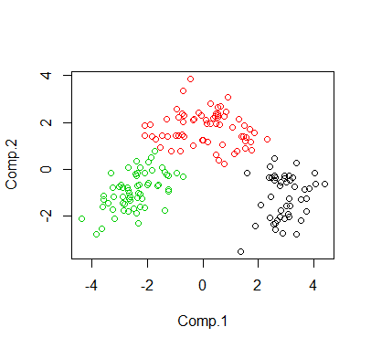
> wine.dat = read.table("wine.dat",header=TRUE)
> cl <- kmeans(wine.dat, 3)
> print(cl$size)
[1] 49 67 62
> 
> # plot in 2D via PCA
> pcafit <- princomp(wine.dat)
> plot(pcafit$scores[,1:2], col = cl$cluster)

Ex 4.1

a&b

The M-step is the same. But for E-step, we use $\hat x_i=x_i+x_u*\frac{p_{ii}+p_{it}}{p_{ii}+p_{it}+p_{tt}}$ and $\hat x_t=x_t+x_u*\frac{p_{tt}}{p_{ii}+p_{it}+p_{tt}}$ to esitmate the expexted genotype frequencies instead $x_i$ and $x_t$ .
Result:

# FINAL ESTIMATE FOR ALLELE PROBABILITIES (p.c, p.i, p.t)
[1] 0.03606708 0.19579915 0.76813377

> #########################################################################
> # x = observed phenotype counts (carbonaria, insularia, typica, i or t)
> # n = expected genotype frequencies (CC, CI, CT, II, IT, TT)
> # p = allele probabilities (carbonaria, insularia, typica)
> # itr = number of iterations
> # allele.e = computes expected genotype frequencies
> # allele.m = computes allele probabilities
> #########################################################################
> 
> ## INITIAL VALUES
> x = c(85, 196, 341, 578)
> n = rep(0,6)
> p = rep(1/3,3)
> itr = 40
> 
> ## EXPECTATION AND MAXIMIZATION FUNCTIONS
> allele.e = function(x,p){
+   n.cc = (x[1]*(p[1]^2))/((p[1]^2)+2*p[1]*p[2]+2*p[1]*p[3])
+   n.ci = (2*x[1]*p[1]*p[2])/((p[1]^2)+2*p[1]*p[2]+2*p[1]*p[3])
+   n.ct = (2*x[1]*p[1]*p[3])/((p[1]^2)+2*p[1]*p[2]+2*p[1]*p[3])
+   x2hat = x[2]+x[4]*((p[2]^2)+2*p[2]*p[3])/((p[2]^2)+2*p[2]*p[3]+p[3]*p[3])
+   x3hat = x[3]+x[4]*(p[3]*p[3])/((p[2]^2)+2*p[2]*p[3]+p[3]*p[3])
+   n.ii = (x2hat*(p[2]^2))/((p[2]^2)+2*p[2]*p[3])
+   n.it = (2*x2hat*p[2]*p[3])/((p[2]^2)+2*p[2]*p[3])
+   n = c(n.cc,n.ci,n.ct,n.ii,n.it,x3hat)
+   return(n)
+ }
> 
> allele.m = function(x,n){
+   p.c = (2*n[1]+n[2]+n[3])/(2*sum(x))
+   p.i = (2*n[4]+n[5]+n[2])/(2*sum(x))
+   p.t = (2*n[6]+n[3]+n[5])/(2*sum(x))
+   p = c(p.c,p.i,p.t)
+   return(p)
+ }
> 
> ## MAIN
> for(i in 1:itr){
+   n = allele.e(x,p)
+   p = allele.m(x,n)
+ }
> 
> ## OUTPUT
> p    # FINAL ESTIMATE FOR ALLELE PROBABILITIES (p.c, p.i, p.t)
[1] 0.03606708 0.19579915 0.76813377

c

Result:

> ## OUTPUT
> sd.hat    # STANDARD ERROR ESTIMATES (pc, pi, pt)
[1] 0.003840308 0.011077418 0.011530716
> cor.hat   # CORRELATION ESTIMATES ({pc,pi}, {pc,pt}, {pi,pt})
[1] -0.03341484 -0.30094901 -0.94955901

Code:

> #########################################################################
> # x = observed phenotype counts (carbonaria, insularia, typica)
> # n = expected genotype frequencies (CC, CI, CT, II, IT, TT)
> # p = allele probabilities (carbonaria, insularia, typica)
> # p.em = em algorithm estimates
> # n.em = em algorithm estimates
> # itr = number of iterations
> # allele.e = computes expected genotype frequencies
> # allele.m = computes allele probabilities
> #########################################################################
> 
> ## INITIAL VALUES
> x = c(85, 196, 341, 578)
> n = rep(0,6)
> itr = 40
> p = c(0.04, 0.19, 0.77)
> p.em = p
> theta = matrix(0,3,3)
> psi = rep(0,3)
> r = matrix(0,3,3)
> 
> ## EXPECTATION AND MAXIMIZATION FUNCTIONS
> allele.e = function(x,p){
+   n.cc = (x[1]*(p[1]^2))/((p[1]^2)+2*p[1]*p[2]+2*p[1]*p[3])
+   n.ci = (2*x[1]*p[1]*p[2])/((p[1]^2)+2*p[1]*p[2]+2*p[1]*p[3])
+   n.ct = (2*x[1]*p[1]*p[3])/((p[1]^2)+2*p[1]*p[2]+2*p[1]*p[3])
+   x2hat = x[2]+x[4]*((p[2]^2)+2*p[2]*p[3])/((p[2]^2)+2*p[2]*p[3]+p[3]*p[3])
+   x3hat = x[3]+x[4]*(p[3]*p[3])/((p[2]^2)+2*p[2]*p[3]+p[3]*p[3])
+   n.ii = (x2hat*(p[2]^2))/((p[2]^2)+2*p[2]*p[3])
+   n.it = (2*x2hat*p[2]*p[3])/((p[2]^2)+2*p[2]*p[3])
+   n = c(n.cc,n.ci,n.ct,n.ii,n.it,x3hat)
+   return(n)
+ }
> 
> allele.m = function(x,n){
+   p.c = (2*n[1]+n[2]+n[3])/(2*sum(x))
+   p.i = (2*n[4]+n[5]+n[2])/(2*sum(x))
+   p.t = (2*n[6]+n[3]+n[5])/(2*sum(x))
+   p = c(p.c,p.i,p.t)
+   return(p)
+ }
> 
> ## COMPUTES EM ALGORITHM ESTIMATES
> for(i in 1:itr){
+   n.em = allele.e(x,p.em)
+   p.em = allele.m(x,n.em)
+ }
> 
> ## INTIALIZES THETA
> for(j in 1:length(p)){
+   theta[,j] = p.em
+   theta[j,j] = p[j]
+ }
> 
> ## MAIN
> for(t in 1:5){
+   n = allele.e(x,p)
+   p.hat = allele.m(x,n)
+   for(j in 1:length(p)){
+     theta[j,j] = p.hat[j]
+     n = allele.e(x,theta[,j])
+     psi = allele.m(x,n)
+     for(i in 1:length(p)){
+       r[i,j] = (psi[i]-p.em[i])/(theta[j,j]-p.em[j])
+     }
+   }
+   p = p.hat
+ }
> 
> ## COMPLETE INFORMATION
> iy.hat=matrix(0,2,2)
> iy.hat[1,1] = ((2*n.em[1]+n.em[2]+n.em[3])/(p.em[1]^2) +
+                  (2*n.em[6]+n.em[3]+n.em[5])/(p.em[3]^2))
> iy.hat[2,2] = ((2*n.em[4]+n.em[5]+n.em[2])/(p.em[2]^2) +
+                  (2*n.em[6]+n.em[3]+n.em[5])/(p.em[3]^2))
> iy.hat[1,2] = iy.hat[2,1] = (2*n.em[6]+n.em[3]+n.em[5])/(p.em[3]^2)
> 
> ## COMPUTES STANDARD ERRORS AND CORRELATIONS
> var.hat = solve(iy.hat)%*%(diag(2)+t(r[-3,-3])%*%solve(diag(2)-t(r[-3,-3])))
> sd.hat = c(sqrt(var.hat[1,1]),sqrt(var.hat[2,2]),sqrt(sum(var.hat)))
> cor.hat = c(var.hat[1,2]/(sd.hat[1]*sd.hat[2]),
+             (-var.hat[1,1]-var.hat[1,2])/(sd.hat[1]*sd.hat[3]),
+             (-var.hat[2,2]-var.hat[1,2])/(sd.hat[2]*sd.hat[3]))
> 
> ## OUTPUT
> sd.hat    # STANDARD ERROR ESTIMATES (pc, pi, pt)
[1] 0.003840308 0.011077418 0.011530716
> cor.hat   # CORRELATION ESTIMATES ({pc,pi}, {pc,pt}, {pi,pt})
[1] -0.03341484 -0.30094901 -0.94955901

d

Result:

> ## OUTPUT
> theta[,1] # EM ESTIMATE FOR ALLELE PROBABILITIES (p.c, p.i, p.t)
[1] 0.03606708 0.19579915 0.76813377
> sd.hat    # STANDARD ERROR ESTIMATES (p.c, p.i, p.t)
[1] 0.003864236 0.012547943 0.012905975
> cor.hat   # CORRELATION ESTIMATES ({p.c,p.i}, {p.c,p.t}, {p.i,p.t})
[1] -0.06000425 -0.24107484 -0.95429228

Code:

> #########################################################################
> # x = observed phenotype counts (carbonaria, insularia, typica)
> # n = expected genotype frequencies (CC, CI, CT, II, IT, TT)
> # p = allele probabilities (carbonaria, insularia, typica)
> # itr = number of iterations
> # theta = allele probabilities for psuedo-data
> # allele.e = computes expected genotype frequencies
> # allele.m = computes allele probabilities
> #########################################################################
> 
> ## INITIAL VALUES
> x = c(85, 196, 341,578)
> n = rep(0,6)
> p = rep(1/3,3)
> itr = 40
> theta = matrix(0,3,10000)
> set.seed(0)
> 
> ## EXPECTATION AND MAXIMIZATION FUNCTIONS
> allele.e = function(x,p){
+   n.cc = (x[1]*(p[1]^2))/((p[1]^2)+2*p[1]*p[2]+2*p[1]*p[3])
+   n.ci = (2*x[1]*p[1]*p[2])/((p[1]^2)+2*p[1]*p[2]+2*p[1]*p[3])
+   n.ct = (2*x[1]*p[1]*p[3])/((p[1]^2)+2*p[1]*p[2]+2*p[1]*p[3])
+   x2hat = x[2]+x[4]*((p[2]^2)+2*p[2]*p[3])/((p[2]^2)+2*p[2]*p[3]+p[3]*p[3])
+   x3hat = x[3]+x[4]*(p[3]*p[3])/((p[2]^2)+2*p[2]*p[3]+p[3]*p[3])
+   n.ii = (x2hat*(p[2]^2))/((p[2]^2)+2*p[2]*p[3])
+   n.it = (2*x2hat*p[2]*p[3])/((p[2]^2)+2*p[2]*p[3])
+   n = c(n.cc,n.ci,n.ct,n.ii,n.it,x3hat)
+   return(n)
+ }
> allele.m = function(x,n){
+   p.c = (2*n[1]+n[2]+n[3])/(2*sum(x))
+   p.i = (2*n[4]+n[5]+n[2])/(2*sum(x))
+   p.t = (2*n[6]+n[3]+n[5])/(2*sum(x))
+   p = c(p.c,p.i,p.t)
+   return(p)
+ }
> 
> ## MAIN
> for(i in 1:itr){
+   n = allele.e(x,p)
+   p = allele.m(x,n)
+ }
> theta[,1] = p
> for(j in 2:10000){
+   n.c = rbinom(1, sum(x), x[1]/sum(x))
+   n.i = rbinom(1, sum(x) - n.c, x[2]/(sum(x)-x[1]))
+   n.t = rbinom(1, sum(x) - n.c - n.i, x[3]/(sum(x)-x[1]-x[2]))
+   n.u = sum(x) - n.c - n.i - n.t
+   x.new = c(n.c, n.i, n.t, n.u)
+   n = rep(0,6)
+   p = rep(1/3,3)
+   for(i in 1:itr){
+     n = allele.e(x.new,p)
+     p = allele.m(x.new,n)
+   }
+   theta[,j] = p
+ }
> 
> sd.hat = c(sd(theta[1,]), sd(theta[2,]), sd(theta[3,]))
> cor.hat = c(cor(theta[1,],theta[2,]), cor(theta[1,],theta[3,]),
+             cor(theta[2,],theta[3,]))
> 
> ## OUTPUT
> theta[,1] # EM ESTIMATE FOR ALLELE PROBABILITIES (p.c, p.i, p.t)
[1] 0.03606708 0.19579915 0.76813377
> sd.hat    # STANDARD ERROR ESTIMATES (p.c, p.i, p.t)
[1] 0.003864236 0.012547943 0.012905975
> cor.hat   # CORRELATION ESTIMATES ({p.c,p.i}, {p.c,p.t}, {p.i,p.t})
[1] -0.06000425 -0.24107484 -0.95429228

e

Output:

> ## OUTPUT
> p     # FINAL ESTIMATE FOR ALLELE PROBABILITIES (p.c, p.i, p.t)
[1] 0.03596147 0.19582060 0.76821793

41e.png-4.2kB

Code:

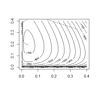
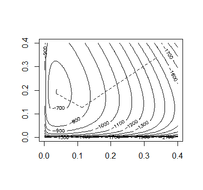
## INITIAL VALUES
x = c(85, 196, 341, 578)
n = rep(0,6)
p = rep(1/3,3)
itr = 40
prob.values = matrix(0,3,itr+1)
prob.values[,1] = p
alpha.default = 2
## FUNCTIONS
allele.e = function(x,p){
  n.cc = (x[1]*(p[1]^2))/((p[1]^2)+2*p[1]*p[2]+2*p[1]*p[3])
  n.ci = (2*x[1]*p[1]*p[2])/((p[1]^2)+2*p[1]*p[2]+2*p[1]*p[3])
  n.ct = (2*x[1]*p[1]*p[3])/((p[1]^2)+2*p[1]*p[2]+2*p[1]*p[3])
  x2hat = x[2]+x[4]*((p[2]^2)+2*p[2]*p[3])/((p[2]^2)+2*p[2]*p[3]+p[3]*p[3])
  x3hat = x[3]+x[4]*(p[3]*p[3])/((p[2]^2)+2*p[2]*p[3]+p[3]*p[3])
  n.ii = (x2hat*(p[2]^2))/((p[2]^2)+2*p[2]*p[3])
  n.it = (2*x2hat*p[2]*p[3])/((p[2]^2)+2*p[2]*p[3])
  n = c(n.cc,n.ci,n.ct,n.ii,n.it,x3hat)
  return(n)
}
allele.l = function(x,p){
  l = ( x[1]*log(2*p[1] - p[1]^2) + x[2]*log(p[2]^2 + 2*p[2]*p[3]) +
          2*x[3]*log(p[3]) + x[4]*log(p[2]^2 + 2*p[2]*p[3]+p[3]^2) )
  return(l)
}
Q.prime = function(n,p){
  da = (2*n[1]+n[2]+n[3])/(p[1]) - (2*n[6]+n[3]+n[5])/(p[3])
  db = (2*n[4]+n[5]+n[2])/(p[2]) - (2*n[6]+n[3]+n[5])/(p[3])
  dQ = c(da,db)
  return(dQ)
}
Q.2prime = function(n,p){
  da2 = -(2*n[1]+n[2]+n[3])/(p[1]^2) - (2*n[6]+n[3]+n[5])/(p[3]^2)
  51
  db2 = -(2*n[4]+n[5]+n[2])/(p[2]^2) - (2*n[6]+n[3]+n[5])/(p[3]^2)
  dab = -(2*n[6]+n[3]+n[5])/(p[3]^2)
  d2Q = matrix(c(da2,dab,dab,db2), nrow=2, byrow=TRUE)
  return(d2Q)
}
## MAIN
l.old = allele.l(x,p)
for(i in 1:itr){
  alpha = alpha.default
  n = allele.e(x,p)
  p.new = p[1:2] - alpha*solve(Q.2prime(n,p))%*%Q.prime(n,p)
  p.new[3] = 1 - p.new[1] - p.new[2]
  if(p.new > 0 && p.new < 1){l.new = allele.l(x,p.new)}
  # REDUCE ALPHA UNTIL A CORRECT STEP IS REACHED
  while(p.new < 0 || p.new > 1 || l.new < l.old){
    alpha = alpha/2
    p.new = p[1:2] - alpha*solve(Q.2prime(n,p))%*%Q.prime(n,p)
    p.new[3] = 1 - p.new[1] - p.new[2]
    if(p.new > 0 && p.new < 1){l.new = allele.l(x,p.new)}
  }
  p = p.new
  prob.values[,i+1] = p
  l.old = l.new
}
## OUTPUT
p     # FINAL ESTIMATE FOR ALLELE PROBABILITIES (p.c, p.i, p.t)
## PLOT OF CONVERGENCE
pb = seq(0.001,0.4,length=100)
c = outer(pb,pb,function(a,b){1-a-b})
pbs = matrix(0,3,10000)
pbs[1,] = rep(pb,100)
pbs[2,] = rep(pb,each=100)
pbs[3,] = as.vector(c)
z = matrix(apply(pbs,2,allele.l,x=x),100,100)
contour(pb,pb,z,nlevels=20)
for(i in 1:itr){
  segments(prob.values[1,i],prob.values[2,i],prob.values[1,i+1],
           prob.values[2,i+1],lty=2)
}

f

Output:

> ## OUTPUT
> p    # FINAL ESTIMATE FOR ALLELE PROBABILITIES (p.c, p.i, p.t)
[1] 0.03606708 0.19579915 0.76813377

41f.png-4.3kB

Code:


## INITIAL VALUES
x = c(85, 196, 341,578)
n = rep(0,6)
p = rep(1/3,3)
itr = 40
prob.values = matrix(0,3,itr+1)
prob.values[,1] = p
alpha.default = 2
## FUNCTIONS
allele.e = function(x,p){
  n.cc = (x[1]*(p[1]^2))/((p[1]^2)+2*p[1]*p[2]+2*p[1]*p[3])
  n.ci = (2*x[1]*p[1]*p[2])/((p[1]^2)+2*p[1]*p[2]+2*p[1]*p[3])
  n.ct = (2*x[1]*p[1]*p[3])/((p[1]^2)+2*p[1]*p[2]+2*p[1]*p[3])
  x2hat = x[2]+x[4]*((p[2]^2)+2*p[2]*p[3])/((p[2]^2)+2*p[2]*p[3]+p[3]*p[3])
  x3hat = x[3]+x[4]*(p[3]*p[3])/((p[2]^2)+2*p[2]*p[3]+p[3]*p[3])
  n.ii = (x2hat*(p[2]^2))/((p[2]^2)+2*p[2]*p[3])
  n.it = (2*x2hat*p[2]*p[3])/((p[2]^2)+2*p[2]*p[3])
  n = c(n.cc,n.ci,n.ct,n.ii,n.it,x3hat)
  return(n)
}
allele.m = function(x,n){
  p.c = (2*n[1]+n[2]+n[3])/(2*sum(x))
  p.i = (2*n[4]+n[5]+n[2])/(2*sum(x))
  p.t = (2*n[6]+n[3]+n[5])/(2*sum(x))
  p = c(p.c,p.i,p.t)
  return(p)
}
allele.l = function(x,p){
  l = ( x[1]*log(2*p[1] - p[1]^2) + x[2]*log(p[2]^2 + 2*p[2]*p[3]) +
          2*x[3]*log(p[3]) + 2*x[4]*log(1-p[1]) )
  return(l)
}
allele.iy = function(n,p){
  iy.hat=matrix(0,2,2)
  iy.hat[1,1] = ((2*n[1]+n[2]+n[3])/(p[1]^2) +
                   (2*n[6]+n[3]+n[5])/(p[3]^2))
  iy.hat[2,2] = ((2*n[4]+n[5]+n[2])/(p[2]^2) +
                   (2*n[6]+n[3]+n[5])/(p[3]^2))
  iy.hat[1,2] = iy.hat[2,1] = (2*n[6]+n[3]+n[5])/(p[3]^2)
  return(iy.hat)
}
allele.l.2prime = function(x,p){
  l.2prime = matrix(0,2,2)
  l.2prime[1,1] = ( (-x[1]*(2-2*p[1])^2)/((2*p[1]-p[1]^2)^2) -
                      2*x[1]/(2*p[1]-p[1]^2) -
                      (4*x[2])/((-2*p[1]-p[2]+2)^2) -
                      2*x[3]/(p[3]^2)
                    -2*x[4]/(1-p[1])^2
                    )
  l.2prime[2,2] = ( (-4*x[2]*p[3]^2)/((p[2]^2 + 2*p[2]*p[3])^2) -
                      2*x[2]/(p[2]^2 + 2*p[2]*p[3]) -
                      2*x[3]/(p[3]^2)
                    )
  l.2prime[1,2] = ((-2*x[2])/((-2*p[1]-p[2]+2)^2) -
                     2*x[3]/(p[3]^2))
  l.2prime[2,1] = l.2prime[1,2]
  return(l.2prime)
}
## MAIN
l.old = allele.l(x,p)
for(i in 1:itr){
  alpha = alpha.default
  n = allele.e(x,p)
  p.em = allele.m(x,n)
  p.new = (p[1:2] - alpha*solve(allele.l.2prime(x,p))%*%
             allele.iy(n,p)%*%(p.em[1:2]-p[1:2]))
  p.new[3] = 1 - p.new[1] - p.new[2]
  if(p.new > 0 && p.new < 1){l.new = allele.l(x,p.new)}
  # REDUCE ALPHA UNTIL A CORRECT STEP IS REACHED
  while(p.new < 0 || p.new > 1 || l.new < l.old){
    alpha = alpha/2
    p.new = (p[1:2] - alpha*solve(allele.l.2prime(x,p))%*%
               allele.iy(n,p)%*%(p.em[1:2]-p[1:2]))
    p.new[3] = 1 - p.new[1] - p.new[2]
    if(p.new > 0 && p.new < 1){l.new = allele.l(x,p.new)}
  }
  p = p.new
  prob.values[,i+1] = p
  l.old = l.new
}
## OUTPUT
p    # FINAL ESTIMATE FOR ALLELE PROBABILITIES (p.c, p.i, p.t)
## PLOT OF CONVERGENCE
pb = seq(0.001,0.4,length=100)
c = outer(pb,pb,function(a,b){1-a-b})
pbs = matrix(0,3,10000)
pbs[1,] = rep(pb,100)
pbs[2,] = rep(pb,each=100)
pbs[3,] = as.vector(c)
z = matrix(apply(pbs,2,allele.l,x=x),100,100)
contour(pb,pb,z,nlevels=20)
for(i in 1:itr){
  segments(prob.values[1,i],prob.values[2,i],prob.values[1,i+1],
           prob.values[2,i+1],lty=2)
}

g

Output:

> ## OUTPUT
> p   # FINAL ESTIMATE FOR ALLELE PROBABILITIES (p.c, p.i, p.t)
[1] 0.03606708 0.19580543 0.76812749

41g.png-4.3kB

Code:

## INITIAL VALUES
x = c(85, 196, 341, 578)
n = rep(0,6)
p = rep(1/3,3)
itr = 20
m = matrix(0,2,2)
b = matrix(0,2,2)
prob.values = matrix(0,3,itr+1)
prob.values[,1] = p
alpha.default = 2
## FUNCTIONS
allele.e = function(x,p){
  n.cc = (x[1]*(p[1]^2))/((p[1]^2)+2*p[1]*p[2]+2*p[1]*p[3])
  n.ci = (2*x[1]*p[1]*p[2])/((p[1]^2)+2*p[1]*p[2]+2*p[1]*p[3])
  n.ct = (2*x[1]*p[1]*p[3])/((p[1]^2)+2*p[1]*p[2]+2*p[1]*p[3])
  x2hat = x[2]+x[4]*((p[2]^2)+2*p[2]*p[3])/((p[2]^2)+2*p[2]*p[3]+p[3]*p[3])
  x3hat = x[3]+x[4]*(p[3]*p[3])/((p[2]^2)+2*p[2]*p[3]+p[3]*p[3])
  n.ii = (x2hat*(p[2]^2))/((p[2]^2)+2*p[2]*p[3])
  n.it = (2*x2hat*p[2]*p[3])/((p[2]^2)+2*p[2]*p[3])
  n = c(n.cc,n.ci,n.ct,n.ii,n.it,x3hat)
  return(n)
}
allele.l = function(x,p){
  l = ( x[1]*log(2*p[1] - p[1]^2) + x[2]*log(p[2]^2 + 2*p[2]*p[3]) +
          2*x[3]*log(p[3]) + 2*x[4]*log(1-p[1]) )
  return(l)
}
Q.prime = function(n,p){
  da = (2*n[1]+n[2]+n[3])/(p[1]) - (2*n[6]+n[3]+n[5])/(p[3])
  db = (2*n[4]+n[5]+n[2])/(p[2]) - (2*n[6]+n[3]+n[5])/(p[3])
  dQ = c(da,db)
  return(dQ)
}
Q.2prime = function(n,p){
  da2 = -(2*n[1]+n[2]+n[3])/(p[1]^2) - (2*n[6]+n[3]+n[5])/(p[3]^2)
  db2 = -(2*n[4]+n[5]+n[2])/(p[2]^2) - (2*n[6]+n[3]+n[5])/(p[3]^2)
  dab = -(2*n[6]+n[3]+n[5])/(p[3]^2)
  d2Q = matrix(c(da2,dab,dab,db2), nrow=2, byrow=TRUE)
  return(d2Q)
}
## MAIN
l.old = allele.l(x,p)
for(i in 1:itr){
  alpha = alpha.default
  n = allele.e(x,p)
  m = Q.2prime(n,p) - b
  p.new = p[1:2] - alpha*solve(m)%*%Q.prime(n,p)
  p.new[3] = 1 - p.new[1] - p.new[2]
  if(p.new > 0 && p.new < 1){l.new = allele.l(x,p.new)}
  # REDUCE ALPHA UNTIL A CORRECT STEP IS REACHED
  while(p.new < 0 || p.new > 1 || l.new < l.old){
    alpha = alpha/2
    p.new = p[1:2] - alpha*solve(m)%*%Q.prime(n,p)
    p.new[3] = 1 - p.new[1] - p.new[2]
    if(p.new > 0 && p.new < 1){l.new = allele.l(x,p.new)}
  }
  at = p.new[1:2]-p[1:2]
  n = allele.e(x,p.new)
  bt = Q.prime(n,p)-Q.prime(n,p.new)
  vt = bt - b%*%at
  ct = as.numeric(1/(t(vt)%*%at))
  b = b + ct*vt%*%t(vt)
  p = p.new
  prob.values[,i+1] = p
  l.old = l.new
}
## OUTPUT
p   # FINAL ESTIMATE FOR ALLELE PROBABILITIES (p.c, p.i, p.t)
## PLOT OF CONVERGENCE
pb = seq(0.001,0.4,length=100)
c = outer(pb,pb,function(a,b){1-a-b})
pbs = matrix(0,3,10000)
pbs[1,] = rep(pb,100)
pbs[2,] = rep(pb,each=100)
pbs[3,] = as.vector(c)
z = matrix(apply(pbs,2,allele.l,x=x),100,100)
contour(pb,pb,z,nlevels=20)
for(i in 1:itr){
  segments(prob.values[1,i],prob.values[2,i],prob.values[1,i+1],
           prob.values[2,i+1],lty=2)
}

h

Accoding to the figures of the above methods, we can tell the Aitken accerlerated EM is the most efficient.

4.5

a

Forward function:
Given $\alpha(i,h)$ for all $h \in H$ . Then for any $h\in H$ , we compute $\alpha(i+1,h) = P(O_{\leq i+1}=o_{\leq i+1}, H_{i+1}=h) \\ = \sum_{h^*\in H} P(O_{\leq i+1}=o_{\leq i+1}, H_{i+1}=h, H_i=h^*) \\ = \sum_{h^*\in H} P(O_{i+1}=o_{i+1}|H_{i+1}=h)P(H_{i+1}=h|H_i=h^*)\\P(O_{\leq i}=o_{\leq i}, H_i=h^*) \\ = \sum_{h^*\in H} \alpha(i,h^*)p(h^*,h)e(h,o_{i+1})$
Backward function:
Given $\beta(i,h)$ for all $h \in H$ . Then for any $h\in H$ , we compute $\beta(i-1,h) = P(O_{>i-1}=o_{>i-1}|H_{i-1}=h) \\ = \sum_{h^*\in H} P(O_{>i-1}=o_{>i-1},H_{i}=h^*|H_{i-1}=h)\\ = \sum_{h^*\in H} P(H_{i}=h^*|H_{i-1}=h)P(O_{>i-1}=o_{>i-1}|H_{i}=h^*)\\ = \sum_{h^*\in H} p(h,h^*)P(O_{>i}=o_{>i}|H_{i}=h^*)P(O_{i}=o_{i}|H_{i}=h^*)\\ = \sum_{h^*\in H} p(h,h^*)e(h^*,o_i)\beta(h^*,i)$

b

$E\{N(h)\} = P(H_0=h|O=o,\theta)=\frac{P(O=o|H_0=h)P(H_0=h)}{P(O=o)} = \\ \frac{P(O_0=o_0|H_0=h)P(O_{>0}=o_{>0}|H_0=h)P(H_0=h)}{P(O=o)} = \\ \frac{P(O_0=o_0,H_0=h)P(O_{>0}=o_{>0}|H_0=h)}{P(O=o)} = \frac{\alpha(0,h)\beta(0,h)}{P(O=o)}$

$E\{N(h,h^*)\} = \sum_{i=0}^{n-1} E(I(H_i=h,H_{i+1}=h^*)|O=o) \\ = \sum_{i=0}^{n-1} P(H_i=h,H_{i+1}=h^*|O=o) \\ = \sum_{i=0}^{n-1} \frac{P(H_i=h,H_{i+1}=h^*,O=o)}{P(O=o)}\\ = \sum_{i=0}^{n-1} \frac{P(H_{i+1}=h^*,O=o|H_i=h)P(H_i=h)}{P(O=o)}\\ = \sum_{i=0}^{n-1} \frac{P(O_{\leq i}=o_{\leq i}|H_i=h)P(H_i=h)P(O_{> i}=o_{> i}|H_{i+1}=h^*)P(H_{i+1}=h^*|H_i=h)}{P(O=o)}\\ = \sum_{i=0}^{n-1} \frac{\alpha(i,h)p(h,h^*)e(h^*,o_{i+1})\beta(i+1,h^*)}{P(O=o)}$

$E\{N(h,o)\} = \sum_{i=0}^{n} E(I(H_i=h,O_i=o)|O=o)\\ = \sum_{i:o_i=o} E(I(H_i=h,O_i=o)|O=o) \\ = \sum_{i:o_i=o} \frac{P(H_i=h,O=o)}{P(O=o|theta)}\\ = \sum_{i:o_i=o} \frac{P(O=o|H_i=h)P(H_i=h)}{P(O=o|theta)}\\ = \sum_{i:o_i=o} \frac{P(O_{\leq i}=o_{\leq i}|H_i=h)P(O_{> i}=o_{> i}|H_i=h)P(H_i=h)}{P(O=o|theta)} \\ = \sum_{i:o_i=o} \frac{\alpha(i,h)\beta(i,h)}{P(O=o|theta)}$

C

The log-likelihood is :
$\sum_hN(h)log\pi(h) +\sum_h\sum_o N(h,o) log e(h,o) +\\ \sum_h\sum_{h^*}N(h,h^*)log p(h,h^*)$

So we can take $N(h),N(h,o)$ and $N(h,h^*)$ as laten variables. The proposed fomular is the according MLE when fixing $N(h),N(h,o)$ and $N(h,h^*)$ .

d

Output:

$pi
[1] 0.5 0.5
$p
     [,1] [,2]
[1,]  0.5  0.5
[2,]  0.5  0.5
$e
     [,1] [,2]
[1,] 0.45 0.55
[2,] 0.45 0.55

Code

x = as.matrix(read.table("coin.dat",header=TRUE))+1
n = 200
pi = c(0.5,0.5)
e = matrix(rep(0.5,4),ncol=2)
p = matrix(rep(0.5,4),ncol=2)
cal_alpha = function(pi,e,p,x)
{
  alpha_new = matrix(rep(0,n*2),ncol=2)
  alpha_new[1,1] = pi[1]*e[1,x[1]]
  alpha_new[1,2] = pi[2]*e[2,x[1]]
  for (i in 2:n)
  {
    alpha_new[i,1] = alpha_new[i-1,1]*p[1,1]*e[1,x[i]] + alpha_new[i-1,2]*p[2,1]*e[1,x[i]]
    alpha_new[i,2] = alpha_new[i-1,1]*p[1,2]*e[2,x[i]] + alpha_new[i-1,2]*p[2,2]*e[2,x[i]]
  }
  return(alpha_new)
}
cal_beta = function(pi,e,p,x)
{
  beta_new = matrix(rep(0,n*2),ncol=2)
  beta_new[n,1] = 1
  beta_new[n,2] = 1
  for (i in (n-1):1)
  {
    beta_new[i,1] = p[1,1]*e[1,x[i+1]]*beta_new[i+1,1] + p[1,2]*e[2,x[i+1]]*beta_new[i+1,2]
    beta_new[i,2] = p[2,1]*e[1,x[i+1]]*beta_new[i+1,1] + p[2,2]*e[2,x[i+1]]*beta_new[i+1,2]
  }
  return(beta_new)
}
estep = function(x,alpha,beta,p,e){
  Nh = c(0,0)
  Nhh = matrix(c(0,0,0,0),ncol=2)
  Nho = matrix(c(0,0,0,0),ncol=2)
  Nh = c(alpha[1,1]*beta[1,1],alpha[1,2]*beta[1,2])
  for(i in 1:2)
    for(j in 1:2)
      for(ii in 1:(n-1))
        Nhh[i,j] = Nhh[i,j]+alpha[ii,i]*p[i,j]*e[j,x[ii+1]]*beta[ii+1,j]
  for(i in 1:2)
    for(j in 1:2){
      for(ii in 1:(n))
        if(x[ii] == j)
        {
          Nho[i,j] = Nho[i,j]+alpha[ii,i]*beta[ii,i]
        }
    }
  return(list(Nh=Nh,Nhh=Nhh,Nho=Nho))
}
mstep = function(Nh,Nhh,Nho){
  new_pi = Nh/sum(Nh)
  new_p = Nhh/rowSums(Nhh)
  new_e = Nho/rowSums(Nho)
  return(list(pi=new_pi,p=new_p,e=new_e))
}
iternum = 10
for(iter in 1:iternum)
{
  alpha = cal_alpha(pi,e,p,x)
  beta = cal_beta(pi,e,p,x)
  estep_list = estep(x,alpha,beta,p,e)
  mstep_list = mstep(estep_list$Nh,estep_list$Nhh,estep_list$Nho)
  pi = mstep_list$pi
  p = mstep_list$p
  e = mstep_list$e
  print(mstep_list)
}

HW 3

Ex 3.1

a

b

Ex 3.8

Ex 4.1

a&b

c

d

e

f

g

h

4.5

a

b

C

d

内容目录