第十二次作业

作业

---

problem5.4

背景

Electric potential
Classical mechanics explores concepts such as force, energy, potential etc. Force and potential energy are directly related. A net force acting on any object will cause it to accelerate. As an object moves in the direction in which the force accelerates it, its potential energy decreases: the gravitational potential energy of a cannonball at the top of a hill is greater than at the base of the hill. As it rolls downhill its potential energy decreases, being translated to motion, inertial (kinetic) energy.

It is possible to define the potential of certain force fields so that the potential energy of an object in that field depends only on the position of the object with respect to the field. Two such force fields are the gravitational field and an electric field (in the absence of time-varying magnetic fields). Such fields must affect objects due to the intrinsic properties of the object (e.g., mass or charge) and the position of the object.

Objects may possess a property known as electric charge and an electric field exerts a force on charged objects. If the charged object has a positive charge the force will be in the direction of the electric field vector at that point while if the charge is negative the force will be in the opposite direction. The magnitude of the force is given by the quantity of the charge multiplied by the magnitude of the electric field vector.

摘要

Exercise 5.4 :
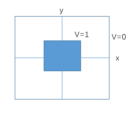
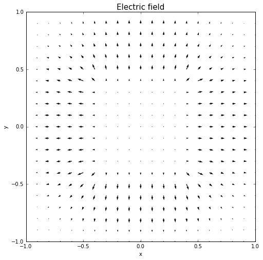
Investigate how the magnitude of the fringing field of the capacitor,that is,the electric field outside the central region of the capcitor in Figure 5.6,varies as a function of plate separation.

正文

解：
假设在z方向上棱柱和金属块时无限延伸的，所以电势分布我们考察平行于x-y平面的某个面即可，电势分布应和z无关。对于中空的部分，因为其中没有电荷，所以描述电势分布用拉普拉斯方程：

$$\frac{\partial^2 V}{\partial x^2}+\frac{\partial^2 V}{\partial y^2}=0$$
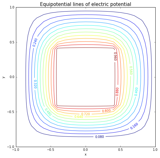
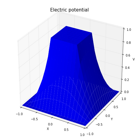
由雅克比法，解为：
$$V(i,j)=\frac{1}{4}[V(i+1,j,k)+V(i-1,j,k)+V(i,j+1,k)+V(i,j-1,k)]$$

代码：

import numpy as np
from pylab import *
from math import *
import mpl_toolkits.mplot3d
# initialize : i represents x, j represents y
V0=[[0 for i in range(21)]for j in range(21)]
for i in range(6,15):
    for j in range(6,15):
        V0[j][i]=1.0# j,i
#check
for j in range(len(V0)):
    for i in range(len(V0[1])):
        print V0[i][j], 
    print
"""
#capacitor initialization
for i in [6]:
    for j in range(6,15):
        V0[j][i]=1.0
for i in [-6]:
    for j in range(6,15):
        V0[j][i]=1.0       
"""
VV=[]
VV.append(V0)
s=0
dx=0.1
#calculate:update V and delta_V
while 1:
    VV.append(V0)
    for i in range(1,len(V0)-1):
        for j in range(1,len(V0[1])-1):
            VV[s+1][i][j]=(VV[s][i+1][j]+VV[s][i-1][j]+\
                          VV[s][i][j+1]+VV[s][i][j-1])/4.0
    for i in range(6,15):
        for j in range(6,15):
            VV[s+1][j][i]=1.0
    for i in [20]:
        for j in range(21):
            VV[s+1][j][i]=0.0
    for i in [-20]:
        for j in range(21):
            VV[s+1][j][i]=0.0
    for j in [20]:
        for i in range(21):
            VV[s+1][j][i]=0.0
    for j in [-20]:
        for i in range(21):
            VV[s+1][j][i]=0.0
"""
    #capacitor calculation
    for i in [6]:
        for j in range(6,15):
            V0[j][i]=1.0
        for i in [-6]:
            for j in range(6,15):
                V0[j][i]=1.0       
"""
#calculate delta_V
    VV[s]=np.array(VV[s])
    VV[s+1]=np.array(VV[s+1])
    dVV=VV[s+1]-VV[s]
    dV=0
    for i in range(1,len(V0)-1):
        for j in range(1,len(V0[1])-1):
            dV=dV+abs(dVV[i][j])
    #print dV 
    s=s+1
    if dV<0.0001 and s>10:
        break
print s
#display final results
#Equipotential lines
figure(figsize=[8,8])
x=np.arange(-1.0,1.01,dx)#-1.0,-0.9,...,1.0
y=np.arange(-1.0,1.01,dx)
X,Y=np.meshgrid(x,y)
CS = contour(X,Y,V,15)
clabel(CS, inline=1, fontsize=10)
xlim(-1,1)
xlabel('x')
ylim(-1,1)
ylabel('y')
title('Equipotential lines of electric potential', fontsize=15)
#3D plot
fig = figure(figsize=[8,8])
ax = fig.add_subplot(111, projection='3d')
ax.plot_surface(X, Y, V,rstride=1, cstride=1,linewidth=0)
ax.set_xlabel('X')
ax.set_ylabel('Y')
ax.set_zlabel('V')
title('Electric potential', fontsize=15)
#Electic field
V=array(VV[-1])
Ex=array(V0)
Ey=array(V0)
for j in range(1,len(V0)-1):
    for i in range(1,len(V0[1])-1):
        Ex[j][i]=-(V[j][i+1]-V[j][i-1])/(2*dx)
        Ey[j][i]=-(V[j+1][i]-V[j-1][i])/(2*dx)
figure(figsize=[8,8])
Q=quiver(X,Y,Ex,Ey,scale=100)
xlim(-1,1)
xlabel('x')
ylim(-1,1)
ylabel('y')
title('Electric field', fontsize=15)
show()

结论

用雅可比方法对拉普拉斯方程进行求解能得到较好的结果。

致谢

感谢《计算物理》课本，以及张同学！