@hanxiaoyang
2016-07-22T16:37:21.000000Z
字数 10425
阅读 3787
斯坦福CS231n学习笔记_(1)_基础介绍
CS231n
作者:寒小阳
时间:2015年11月。
出处:http://blog.csdn.net/han_xiaoyang/article/details/49876119
声明:版权所有,转载请注明出处,谢谢。
1.背景
计算机视觉/computer vision是一个火了N年的topic。持续化升温的原因也非常简单:在搜索/影像内容理解/医学应用/地图识别等等领域应用太多,大家都有一个愿景『让计算机能够像人一样去"看"一张图片,甚至"读懂"一张图片』。
有几个比较重要的计算机视觉任务,比如图片的分类,物体识别,物体定位于检测等等。而近年来的神经网络/深度学习使得上述任务的准确度有了非常大的提升。加之最近做了几个不大不小的计算机视觉上的项目,爱凑热闹的博主自然不打算放过此领域,也边学边做点笔记总结,写点东西,写的不正确的地方,欢迎大家提出和指正。
2.基础知识
为了简单易读易懂,这个课程笔记系列中绝大多数的代码都使用python完成。这里稍微介绍一下python和Numpy/Scipy(python中的科学计算包)的一些基础。
2.1 python基础
python是一种长得像伪代码,具备高可读性的编程语言。
优点挺多:可读性相当好,写起来也简单,所想立马可以转为实现代码,且社区即为活跃,可用的package相当多;缺点:效率一般。
2.1.1 基本数据类型
最常用的有数值型(Numbers),布尔型(Booleans)和字符串(String)三种。
- 数值型(Numbers)
可进行简单的运算,如下:
x = 5print type(x) # Prints "<type 'int'>"print x # Prints "5"print x + 1 # 加; prints "6"print x - 1 # 减; prints "4"print x * 2 # 乘; prints "10"print x ** 2 # 幂; prints "25"x += 1 #自加print x # Prints "6"x *= 2 #自乘print x # Prints "12"y = 2.5print type(y) # Prints "<type 'float'>"print y, y + 1, y * 2, y ** 2 # Prints "2.5 3.5 5.0 6.25"
PS:python中没有x++ 和 x-- 操作
- 布尔型(Booleans)
包含True False和常见的与或非操作
t = Truef = Falseprint type(t) # Prints "<type 'bool'>"print t and f # 逻辑与; prints "False"print t or f # 逻辑或; prints "True"print not t # 逻辑非; prints "False"print t != f # XOR; prints "True"
- 字符串型(String)
字符串可以用单引号/双引号/三引号声明
hello = 'hello'world = "world"print hello # Prints "hello"print len(hello) # 字符串长度; prints "5"hw = hello + ' ' + world # 字符串连接print hw # prints "hello world"hw2015 = '%s %s %d' % (hello, world, 2015) # 格式化字符串print hw2015 # prints "hello world 2015"
字符串对象有很有有用的函数:
s = "hello"print s.capitalize() # 首字母大写; prints "Hello"print s.upper() # 全大写; prints "HELLO"print s.rjust(7) # 以7为长度右对齐,左边补空格; prints " hello"print s.center(7) # 居中补空格; prints " hello "print s.replace('l', '(ell)') # 字串替换;prints "he(ell)(ell)o"print ' world '.strip() # 去首位空格; prints "world"
2.1.2 基本容器
- 列表/List
和数组类似的一个东东,不过可以包含不同类型的元素,同时大小也是可以调整的。
xs = [3, 1, 2] # 创建print xs, xs[2] # Prints "[3, 1, 2] 2"print xs[-1] # 第-1个元素,即最后一个xs[2] = 'foo' # 下标从0开始,这是第3个元素print xs # 可以有不同类型,Prints "[3, 1, 'foo']"xs.append('bar') # 尾部添加一个元素print xs # Printsx = xs.pop() # 去掉尾部的元素print x, xs # Prints "bar [3, 1, 'foo']"
列表最常用的操作有:
切片/slicing
即取子序列/一部分元素,如下:
nums = range(5) # 从1到5的序列print nums # Prints "[0, 1, 2, 3, 4]"print nums[2:4] # 下标从2到4-1的元素 prints "[2, 3]"print nums[2:] # 下标从2到结尾的元素print nums[:2] # 从开头到下标为2-1的元素 [0, 1]print nums[:] # 恩,就是全取出来了print nums[:-1] # 从开始到第-1个元素(最后的元素)nums[2:4] = [8, 9] # 对子序列赋值print nums # Prints "[0, 1, 8, 8, 4]"
循环/loops
即遍历整个list,做一些操作,如下:
animals = ['cat', 'dog', 'monkey']for animal in animals:print animal# 依次输出 "cat", "dog", "monkey",每个一行.
可以用enumerate取出元素的同时带出下标
animals = ['cat', 'dog', 'monkey']for idx, animal in enumerate(animals):print '#%d: %s' % (idx + 1, animal)# 输出 "#1: cat", "#2: dog", "#3: monkey",一个一行。
List comprehension
这个相当相当相当有用,在很长的list生成过程中,效率完胜for循环:
# for 循环nums = [0, 1, 2, 3, 4]squares = []for x in nums:squares.append(x ** 2)print squares # Prints [0, 1, 4, 9, 16]# list comprehensionnums = [0, 1, 2, 3, 4]squares = [x ** 2 for x in nums]print squares # Prints [0, 1, 4, 9, 16]
你猜怎么着,list comprehension也是可以加多重条件的:
nums = [0, 1, 2, 3, 4]even_squares = [x ** 2 for x in nums if x % 2 == 0]print even_squares # Prints "[0, 4, 16]"
- 字典/Dict
和Java中的Map一样的东东,用于存储key-value对:
d = {'cat': 'cute', 'dog': 'furry'} # 创建print d['cat'] # 根据key取出valueprint 'cat' in d # 判断是否有'cat'这个keyd['fish'] = 'wet' # 添加元素print d['fish'] # Prints "wet"# print d['monkey'] # KeyError: 'monkey'非本字典的keyprint d.get('monkey', 'N/A') # 有key返回value,无key返回"N/A"print d.get('fish', 'N/A') # prints "wet"del d['fish'] # 删除某个key以及对应的valueprint d.get('fish', 'N/A') # prints "N/A"
对应list的那些操作,你在dict里面也能找得到:
循环/loops
# for循环d = {'person': 2, 'cat': 4, 'spider': 8}for animal in d:legs = d[animal]print 'A %s has %d legs' % (animal, legs)# Prints "A person has 2 legs", "A spider has 8 legs", "A cat has 4 legs"# 通过iteritemsd = {'person': 2, 'cat': 4, 'spider': 8}for animal, legs in d.iteritems():print 'A %s has %d legs' % (animal, legs)# Prints "A person has 2 legs", "A spider has 8 legs", "A cat has 4 legs"
# Dictionary comprehensionnums = [0, 1, 2, 3, 4]even_num_to_square = {x: x ** 2 for x in nums if x % 2 == 0}print even_num_to_square # Prints "{0: 0, 2: 4, 4: 16}"
- 元组/turple
本质上说,还是一个list,只不过里面的每个元素都是一个两元组对。
d = {(x, x + 1): x for x in range(10)} # 创建t = (5, 6) # Create a tupleprint type(t) # Prints "<type 'tuple'>"print d[t] # Prints "5"print d[(1, 2)] # Prints "1"
2.1.3 函数
用def可以定义一个函数:
def sign(x):if x > 0:return 'positive'elif x < 0:return 'negative'else:return 'zero'for x in [-1, 0, 1]:print sign(x)# Prints "negative", "zero", "positive"
def hello(name, loud=False):if loud:print 'HELLO, %s' % name.upper()else:print 'Hello, %s!' % namehello('Bob') # Prints "Hello, Bob"hello('Fred', loud=True) # Prints "HELLO, FRED!"
- 类/Class
python里面的类定义非常的直接和简洁:
class Greeter:# Constructordef __init__(self, name):self.name = name # Create an instance variable# Instance methoddef greet(self, loud=False):if loud:print 'HELLO, %s!' % self.name.upper()else:print 'Hello, %s' % self.nameg = Greeter('Fred') # Construct an instance of the Greeter classg.greet() # Call an instance method; prints "Hello, Fred"g.greet(loud=True) # Call an instance method; prints "HELLO, FRED!"
2.2.NumPy基础
NumPy是Python的科学计算的一个核心库。它提供了一个高性能的多维数组(矩阵)对象,可以完成在其之上的很多操作。很多机器学习中的计算问题,把数据vectorize之后可以进行非常高效的运算。
2.2.1 数组
一个NumPy数组是一些类型相同的元素组成的类矩阵数据。用list或者层叠的list可以初始化:
import numpy as npa = np.array([1, 2, 3]) # 一维Numpy数组print type(a) # Prints "<type 'numpy.ndarray'>"print a.shape # Prints "(3,)"print a[0], a[1], a[2] # Prints "1 2 3"a[0] = 5 # 重赋值print a # Prints "[5, 2, 3]"b = np.array([[1,2,3],[4,5,6]]) # 二维Numpy数组print b.shape # Prints "(2, 3)"print b[0, 0], b[0, 1], b[1, 0] # Prints "1 2 4"
生成一些特殊的Numpy数组(矩阵)时,我们有特定的函数可以调用:
import numpy as npa = np.zeros((2,2)) # 全0的2*2 Numpy数组print a # Prints "[[ 0. 0.]# [ 0. 0.]]"b = np.ones((1,2)) # 全1 Numpy数组print b # Prints "[[ 1. 1.]]"c = np.full((2,2), 7) # 固定值Numpy数组print c # Prints "[[ 7. 7.]# [ 7. 7.]]"d = np.eye(2) # 2*2 对角Numpy数组print d # Prints "[[ 1. 0.]# [ 0. 1.]]"e = np.random.random((2,2)) # 2*2 的随机Numpy数组print e # 随机输出
2.2.2 Numpy数组索引与取值
可以通过像list一样的分片/slicing操作取出需要的数值部分。
import numpy as np# 创建如下的3*4 Numpy数组# [[ 1 2 3 4]# [ 5 6 7 8]# [ 9 10 11 12]]a = np.array([[1,2,3,4], [5,6,7,8], [9,10,11,12]])# 通过slicing取出前两行的2到3列:# [[2 3]# [6 7]]b = a[:2, 1:3]# 需要注意的是取出的b中的数据实际上和a的这部分数据是同一份数据.print a[0, 1] # Prints "2"b[0, 0] = 77 # b[0, 0] 和 a[0, 1] 是同一份数据print a[0, 1] # a也被修改了,Prints "77"
import numpy as npa = np.array([[1,2,3,4], [5,6,7,8], [9,10,11,12]])row_r1 = a[1, :] # a 的第二行row_r2 = a[1:2, :] # 同上print row_r1, row_r1.shape # Prints "[5 6 7 8] (4,)"print row_r2, row_r2.shape # Prints "[[5 6 7 8]] (1, 4)"col_r1 = a[:, 1]col_r2 = a[:, 1:2]print col_r1, col_r1.shape # Prints "[ 2 6 10] (3,)"print col_r2, col_r2.shape # Prints "[[ 2]# [ 6]# [10]] (3, 1)"
还可以这么着取:
import numpy as npa = np.array([[1,2], [3, 4], [5, 6]])# 取出(0,0) (1,1) (2,0)三个位置的值print a[[0, 1, 2], [0, 1, 0]] # Prints "[1 4 5]"# 和上面一样print np.array([a[0, 0], a[1, 1], a[2, 0]]) # Prints "[1 4 5]"# 取出(0,1) (0,1) 两个位置的值print a[[0, 0], [1, 1]] # Prints "[2 2]"# 同上print np.array([a[0, 1], a[0, 1]]) # Prints "[2 2]"
我们还可以通过条件得到bool型的Numpy数组结果,再通过这个数组取出符合条件的值,如下:
import numpy as npa = np.array([[1,2], [3, 4], [5, 6]])bool_idx = (a > 2) # 判定a大于2的结果矩阵print bool_idx # Prints "[[False False]# [ True True]# [ True True]]"# 再通过bool_idx取出我们要的值print a[bool_idx] # Prints "[3 4 5 6]"# 放在一起我们可以这么写print a[a > 2] # Prints "[3 4 5 6]"
Numpy数组的类型
import numpy as npx = np.array([1, 2])print x.dtype # Prints "int64"x = np.array([1.0, 2.0])print x.dtype # Prints "float64"x = np.array([1, 2], dtype=np.int64) # 强制使用某个typeprint x.dtype # Prints "int64"
2.2.3 Numpy数组的运算
矩阵的加减开方和(元素对元素)乘除如下:
import numpy as npx = np.array([[1,2],[3,4]], dtype=np.float64)y = np.array([[5,6],[7,8]], dtype=np.float64)# [[ 6.0 8.0]# [10.0 12.0]]print x + yprint np.add(x, y)# [[-4.0 -4.0]# [-4.0 -4.0]]print x - yprint np.subtract(x, y)# 元素对元素,点对点的乘积# [[ 5.0 12.0]# [21.0 32.0]]print x * yprint np.multiply(x, y)# 元素对元素,点对点的除法# [[ 0.2 0.33333333]# [ 0.42857143 0.5 ]]print x / yprint np.divide(x, y)# 开方# [[ 1. 1.41421356]# [ 1.73205081 2. ]]print np.sqrt(x)
矩阵的内积是通过下列方法计算的:
import numpy as npx = np.array([[1,2],[3,4]])y = np.array([[5,6],[7,8]])v = np.array([9,10])w = np.array([11, 12])# 向量内积,得到 219print v.dot(w)print np.dot(v, w)# 矩阵乘法,得到 [29 67]print x.dot(v)print np.dot(x, v)# 矩阵乘法# [[19 22]# [43 50]]print x.dot(y)print np.dot(x, y)
特别特别有用的一个操作是,sum/求和(对某个维度):
import numpy as npx = np.array([[1,2],[3,4]])print np.sum(x) # 整个矩阵的和,得到 "10"print np.sum(x, axis=0) # 每一列的和 得到 "[4 6]"print np.sum(x, axis=1) # 每一行的和 得到 "[3 7]"
还有一个经常会用到操作是矩阵的转置,在Numpy数组里用.T实现:
import numpy as npx = np.array([[1,2], [3,4]])print x # Prints "[[1 2]# [3 4]]"print x.T # Prints "[[1 3]# [2 4]]"# 1*n的Numpy数组,用.T之后其实啥也没做:v = np.array([1,2,3])print v # Prints "[1 2 3]"print v.T # Prints "[1 2 3]"
2.2.4 Broadcasting
Numpy还有一个非常牛逼的机制,你想想,如果你现在有一大一小俩矩阵,你想使用小矩阵在大矩阵上做多次操作。额,举个例子好了,假如你想将一个1*n的矩阵,加到m*n的矩阵的每一行上:
#你如果要用for循环实现是酱紫的(下面用y的原因是,你不想改变原来的x)import numpy as npx = np.array([[1,2,3], [4,5,6], [7,8,9], [10, 11, 12]])v = np.array([1, 0, 1])y = np.empty_like(x) # 设置一个和x一样维度的Numpy数组y# 逐行相加for i in range(4):y[i, :] = x[i, :] + v# 恩,y就是你想要的了# [[ 2 2 4]# [ 5 5 7]# [ 8 8 10]# [11 11 13]]print y
#上一种方法如果for的次数非常多,会很慢,于是我们改进了一下import numpy as npx = np.array([[1,2,3], [4,5,6], [7,8,9], [10, 11, 12]])v = np.array([1, 0, 1])vv = np.tile(v, (4, 1)) # 变形,重复然后叠起来print vv # Prints "[[1 0 1]# [1 0 1]# [1 0 1]# [1 0 1]]"y = x + vv # 相加print y # Prints "[[ 2 2 4# [ 5 5 7]# [ 8 8 10]# [11 11 13]]"
#其实因为Numpy的Broadcasting,你可以直接酱紫操作import numpy as npx = np.array([[1,2,3], [4,5,6], [7,8,9], [10, 11, 12]])v = np.array([1, 0, 1])y = x + v # 直接加!!!print y # Prints "[[ 2 2 4]# [ 5 5 7]# [ 8 8 10]# [11 11 13]]"
更多Broadcasting的例子请看下面:
import numpy as npv = np.array([1,2,3]) # v has shape (3,)w = np.array([4,5]) # w has shape (2,)# 首先把v变成一个列向量# v现在的形状是(3, 1);# 作用在w上得到的结果形状是(3, 2),如下# [[ 4 5]# [ 8 10]# [12 15]]print np.reshape(v, (3, 1)) * w# 逐行相加x = np.array([[1,2,3], [4,5,6]])# 得到如下结果:# [[2 4 6]# [5 7 9]]print x + v# 先逐行相加再转置,得到以下结果:# [[ 5 6 7]# [ 9 10 11]]print (x.T + w).T# 恩,也可以这么做print x + np.reshape(w, (2, 1))
2.3 SciPy
Numpy提供了一个非常方便操作和计算的高维向量对象,并提供基本的操作方法,而Scipy是在Numpy的基础上,提供很多很多的函数和方法去直接完成你需要的矩阵操作。有兴趣可以浏览Scipy方法索引查看具体的方法,函数略多,要都记下来有点困难,随用随查吧。
向量距离计算
需要特别拎出来说一下的是,向量之间的距离计算,这个Scipy提供了很好的接口scipy.spatial.distance.pdist:
import numpy as npfrom scipy.spatial.distance import pdist, squareform# [[0 1]# [1 0]# [2 0]]x = np.array([[0, 1], [1, 0], [2, 0]])print x# 计算矩阵每一行和每一行之间的欧氏距离# d[i, j] 是 x[i, :] 和 x[j, :] 之间的距离,# 结果如下:# [[ 0. 1.41421356 2.23606798]# [ 1.41421356 0. 1. ]# [ 2.23606798 1. 0. ]]d = squareform(pdist(x, 'euclidean'))print d
2.4 Matplotlib
这是python中的一个作图工具包。如果你熟悉matlab的语法的话,应该会用得挺顺手。可以通过matplotlib.pyplot.plot了解更多绘图相关的设置和参数。
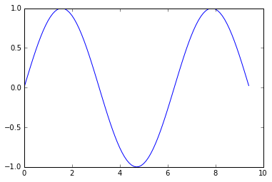
import numpy as npimport matplotlib.pyplot as plt# 计算x和对应的sin值作为yx = np.arange(0, 3 * np.pi, 0.1)y = np.sin(x)# 用matplotlib绘出点的变化曲线plt.plot(x, y)plt.show() # 只有调用plt.show()之后才能显示
结果如下:
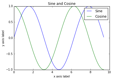
# 在一个图中画出2条曲线import numpy as npimport matplotlib.pyplot as plt# 计算x对应的sin和cos值x = np.arange(0, 3 * np.pi, 0.1)y_sin = np.sin(x)y_cos = np.cos(x)# 用matplotlib作图plt.plot(x, y_sin)plt.plot(x, y_cos)plt.xlabel('x axis label')plt.ylabel('y axis label')plt.title('Sine and Cosine')plt.legend(['Sine', 'Cosine'])plt.show()
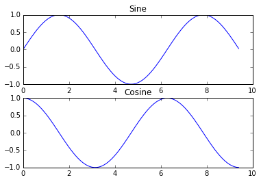
# 用subplot分到子图里import numpy as npimport matplotlib.pyplot as plt# 得到x对应的sin和cos值x = np.arange(0, 3 * np.pi, 0.1)y_sin = np.sin(x)y_cos = np.cos(x)# 2*1个子图,第一个位置.plt.subplot(2, 1, 1)# 画第一个子图plt.plot(x, y_sin)plt.title('Sine')# 画第2个子图plt.subplot(2, 1, 2)plt.plot(x, y_cos)plt.title('Cosine')plt.show()
2.5 简单图片读写
可以使用imshow来显示图片。
import numpy as npfrom scipy.misc import imread, imresizeimport matplotlib.pyplot as pltimg = imread('/Users/HanXiaoyang/Comuter_vision/computer_vision.jpg')img_tinted = img * [1, 0.95, 0.9]# 显示原始图片plt.subplot(1, 2, 1)plt.imshow(img)# 显示调色后的图片plt.subplot(1, 2, 2)plt.imshow(np.uint8(img_tinted))plt.show()

