electric potentials and fields:Laplace's equation

abstract

The partial differential equation is of physicists' great interest for its widely applicaiton in decribing physical systems. Jacobi method and simultaneous over relaxation method are two algrithm that keep a balance of the simplicity for comprehension and accuracy of computation. Here in this passage,we are going to discuss the relation and difference with differnet methods in tackling same problem.
key words:relaxation algorithm,jacobi method,Gauss-seidel method,SOR,Laplace'squation

background

1.about electrical field
An electric field is a vector field that associates to each point in space the Coulomb force that would be experienced per unit of electric charge, by an infinitesimal test charge at that point.1 Electric fields converge and diverge at electric charges and can be induced by time-varying magnetic fields. The electric field combines with the magnetic field to form the electromagnetic field
Laplace's equation(in region of space do not contain any elctric charges):
$\Delta V=\frac{\partial^2V}{\partial^2x}+\frac{\partial^2V}{\partial^2 y}+\frac{\partial^2V}{\partial^2 z}=0$
2.numerical algorithm:relaxation algorithm
1.jacobi method
In numerical linear algebra, the Jacobi method (or Jacobi iterative method) is an algorithm for determining the solutions of a diagonally dominant system of linear equations. Each diagonal element is solved for, and an approximate value is plugged in. The process is then iterated until it converges.
Particularly,in our dicussion in this passage,Jacobi Method can be easily expressed as below:

$V_{new}(i,j)=\frac{1}{4}[V_{old}(i+1,j)+V_{old}(i-1,j)+V_{old}(i,j+1)+V_{old}(i,j-1)]$
2.Gauss-seidel method
In numerical linear algebra, the Gauss–Seidel method, also known as the Liebmann method or the method of successive displacement, is an iterative method used to solve a linear system of equations. It is named after the German mathematicians Carl Friedrich Gauss and Philipp Ludwig von Seidel, and is similar to the Jacobi method.
Particularly,in our dicussion in this passage,Gauss-Seidel Method can be easily expressed as below:
$V_{new}(i,j)=\frac{1}{4}[V_{old}(i+1,j)+V_{new}(i-1,j)+V_{old}(i,j+1)+V_{new}(i,j-1)]$
3.SOR:Simulatneous over-relaxation:
With this method ,the problem of relatively low convergence rate can be easily solved.Let $V^*(i,j)$ be the new value of calculated.Then the change of $V$ is represented as:

$\Delta V(i,j)=V^* (i,j)-V_{old}(i,j)$
However,we have seen in our previous examples that this choice of $\Delta V(i,j)$ is too conservative.So to speed up convergence we will change the potential by a larger amount calculated according to:
$V_{new}(i,j)=\alpha \Delta V(i,j)+V_{old}(i,j)$
where $\alpha$ is a factor that measures how much we "over-relax".Choosing $\alpha=1$ tuekds the Gauss-Seidel method.It turns out that if $\alpha>=2$ , the method does bit converge.The best choice of $\alpha$ is:

$\alpha\approx\frac{2}{1+\pi/L}$

main body

import math
import matplotlib.pyplot as plt
from mpl_toolkits.mplot3d import Axes3D 
import numpy as np
from matplotlib import cm
from matplotlib.ticker import LinearLocator, FormatStrFormatter
class ef:
    #初始化创建二维n*n全为0的矩阵,在后面的函数中通过修改矩阵中元素的值来构建不同的电场
    def __init__(self,alpha=1,n=20):
        self.n=n
        self.field=[[0]*(self.n) for i in range(self.n)]
    #教材figure5.2所示电场
    def field1(self):
        self.field[0]=np.linspace(-1,1,self.n)
        self.field[-1]=np.linspace(-1,1,self.n)
        for k in range(1,self.n-1):
            self.field[k][0]=-1
            self.field[k][-1]=1
        self.kk=1
        while(1):
            self.kk+=1
            for i in range(1,self.n-1):
                for j in range(1,self.n-1):
                    self.field[i][j]=(self.field[i+1][j]+self.field[i-1][j]+self.field[i][j+1]+self.field[i][j-1])/4
            if self.kk>1000:
                break
    #教材figure5.4所示电场
    def field2(self):
        for i in range(int(self.n/4),int(self.n*3/4)):
            for j in range(int(self.n/4),int(self.n*3/4)):
                self.field[i][j]=1
        self.kk=1
        while(1):
            self.kk+=1
            for i in range(1,self.n-1):
                for j in range(1,self.n-1):
                    if int(self.n/4)<=i<=int(self.n*3/4) and int(self.n/4)<=j<=int(self.n*3/4):
                        self.field[i][j]=1
                    else:
                        self.field[i][j]=(self.field[i+1][j]+self.field[i-1][j]+self.field[i][j+1]+self.field[i][j-1])/4
            if self.kk>1000:
                break
    #教材figure5.6所示电场
    def field3(self):
        for i in range(1,self.n-1):
            for j in range(1,self.n-1):
                if j==int(self.n/4) and i>=self.n/4 and i<=self.n*3/4:
                    self.field[i][j]=1
                elif j==int(self.n*3/4) and i>=self.n/4 and i<=self.n*3/4:
                    self.field[i][j]=-1
        self.kk=1
        while(1):
            self.kk+=1
            for i in range(1,self.n-1):
                for j in range(1,self.n-1):
                    if j==int(self.n/4) and i>=self.n/4 and i<=self.n*3/4:
                        self.field[i][j]=1
                    elif j==int(self.n*3/4) and i>=self.n/4 and i<=self.n*3/4:
                        self.field[i][j]=-1
                    else:
                        self.field[i][j]=(self.field[i+1][j]+self.field[i-1][j]+self.field[i][j+1]+self.field[i][j-1])/4
            if self.kk>5000:
                break
    def show_field(self):
        fig = plt.figure()  
        ax = Axes3D(fig)
        X=np.linspace(-1,1,self.n)
        Y=np.linspace(-1,1,self.n)
        X, Y = np.meshgrid(X, Y)
        Z=self.field
        ax.plot_surface(X, Y, Z, rstride=1, cstride=1, cmap=plt.cm.hot)  
        ax.contourf(X, Y, Z, zdir='z', offset=-2, cmap=plt.cm.hot)  
        ax.set_zlim(-2,2) 
a=ef()
a.field2()
a.show_field()

a simple example of relaxation algorithm
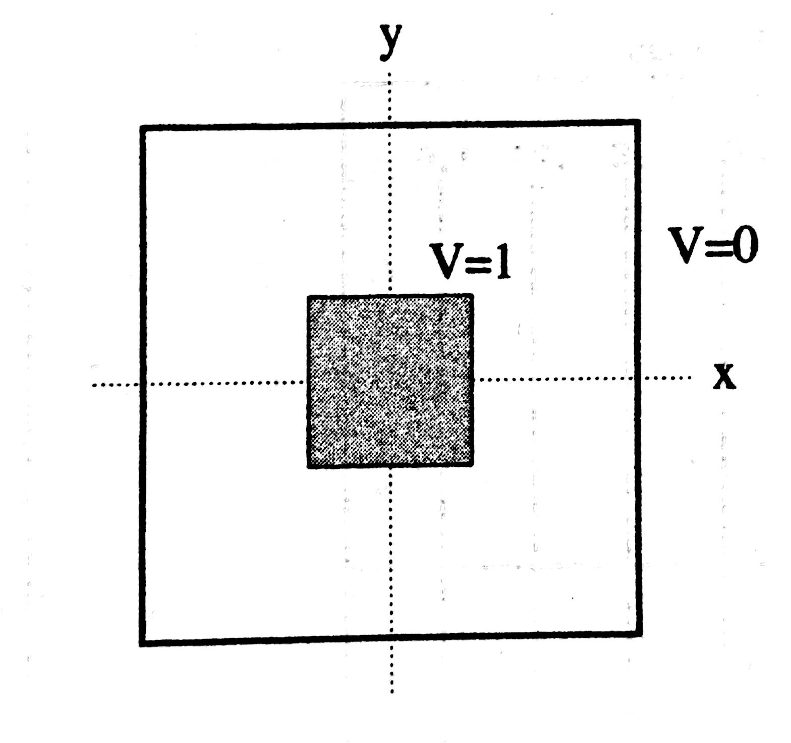
2.Electric potemtial and field inside the prism
3.electric potential of capacitor plates

acknowledgement

Nicholas J.Giodano's computational physics.
csdn-皮皮blog
help of 陆文龙