计算物理第九次作业

作者：夏海峰 学号：2013301020094

摘要

       本次主要研究混沌现象。混沌是自然界普遍存在的现象。混沌现象是指发生在确定性系统中的貌似随机的不规则运动，一个确定性理论描述的系统，其行为却表现为不确定性一不可重复、不可预测，这就是混沌现象。进一步研究表明，混沌是非线性动力系统的固有特性，是非线性系统普遍存在的现象。牛顿确定性理论能够充分处理的多为线性系统，而线性系统大多是由非线性系统简化来的。因此，在现实生活和实际工程技术问题中，混沌是无处不在的。

• 研究起源:
         1963年，Lorenz在《大气科学》杂志上发表了“决定性的非周期流”一文，指出在气候不能精确重演与长期天气预报者无能为力之间必然存在着一种联系，这就是非周期与不可预见性之间的联系。他还发现了混沌现象“对初始条件的极端敏感性”。这可以生动的用“蝴蝶效应”来比喻：在做气象预报时，只要一只蝴蝶扇一下翅膀，这一扰动，就会在很远的另一个地方造成非常大的差异，将使长时间的预测无法进行。
         在60年代研究的基础上，混沌学的研究开始进入高潮。1971年，科学家在耗散系统中正式的引入了奇异吸引子的概念（如Henon吸引子、Lorenz吸引子)。1975年，J.York和T.Y lie提出了混沌的科学概念。整个70年代中期，人们不但在理论上对混沌做更深层次的研究，而且努力在实验室中找寻奇异吸引子。J.York在他的著名论文“周期3意味着混沌”中，指出：在任何一维系统中，只要出现周期3，则该系统也能出现其他长度的周期，也能呈现完全的混沌。
         在确定性的系统中发现混沌，改变了人们过去一直认为宇宙是一个可以预测的系统的看法。用决定论的方程，找不到稳定的模式，得到的却是随机的结果，彻底打破了拉普拉斯决定论式的可预测性的幻想。但人们同时发现到过去许多曾被认为是噪声的信号，其实是一些简单的规则生成的。这些包含内在规则的“噪声”不同于真正的噪声，它们的这种规则是完全可以应用的。

混沌现象

       用Euler-Cromer方法模拟计算如下驱动力下的混沌现象：

$$\frac {d^2 \theta}{dt^2}=-\frac{g}{l}sin(\theta)-q\frac {d\theta}{dt}+F_Dsin(\Omega _D t)$$
       将上式转化为两个一阶线性常微分方程：
$$\frac {d\omega}{dt}=-\frac {g}{l}\sin (\theta)-q\frac {d \theta}{dt}+F_D\sin(\Omega_D t)$$
$$\frac {d\omega}{dt}=\omega$$

• 由以上两式可得出Euler-Cromer方法的具体数值计算方法：
  $$\omega_{i+1}=\omega_i-\left[(g/l) \sin \theta_i-q\omega_i+F_D\sin(\Omega_Dt) \right]$$
  $$\theta_{i+1}=\theta_i+\omega_{i+1}\Delta t$$
  $$t_{i+1}=t_i+\Delta t$$

• 驱动力变化时摆的运动情况变化如下图所示：
  程序
  

• 参数q变化时摆的运动情况变化如下图所示：
  程序
  

作业3.12题

• 3.12
  In constructing the Poincaré section in Figure 3.9 we plotted points only at times that were in phase with the drive force; that is, at times $t \approx 2\pi n/\Omega_D$, where n is an integer. At these values of t the driving force passed through zero [see (3.18)]. However, we could just as easily have chosen to make the plot at times corresponding to a maximum of the drive force, or at times $\pi /4$ out-of-phase with this force, etc. Construct the Poincaré sections for these cases and compare them with Figure 3.9.

程序

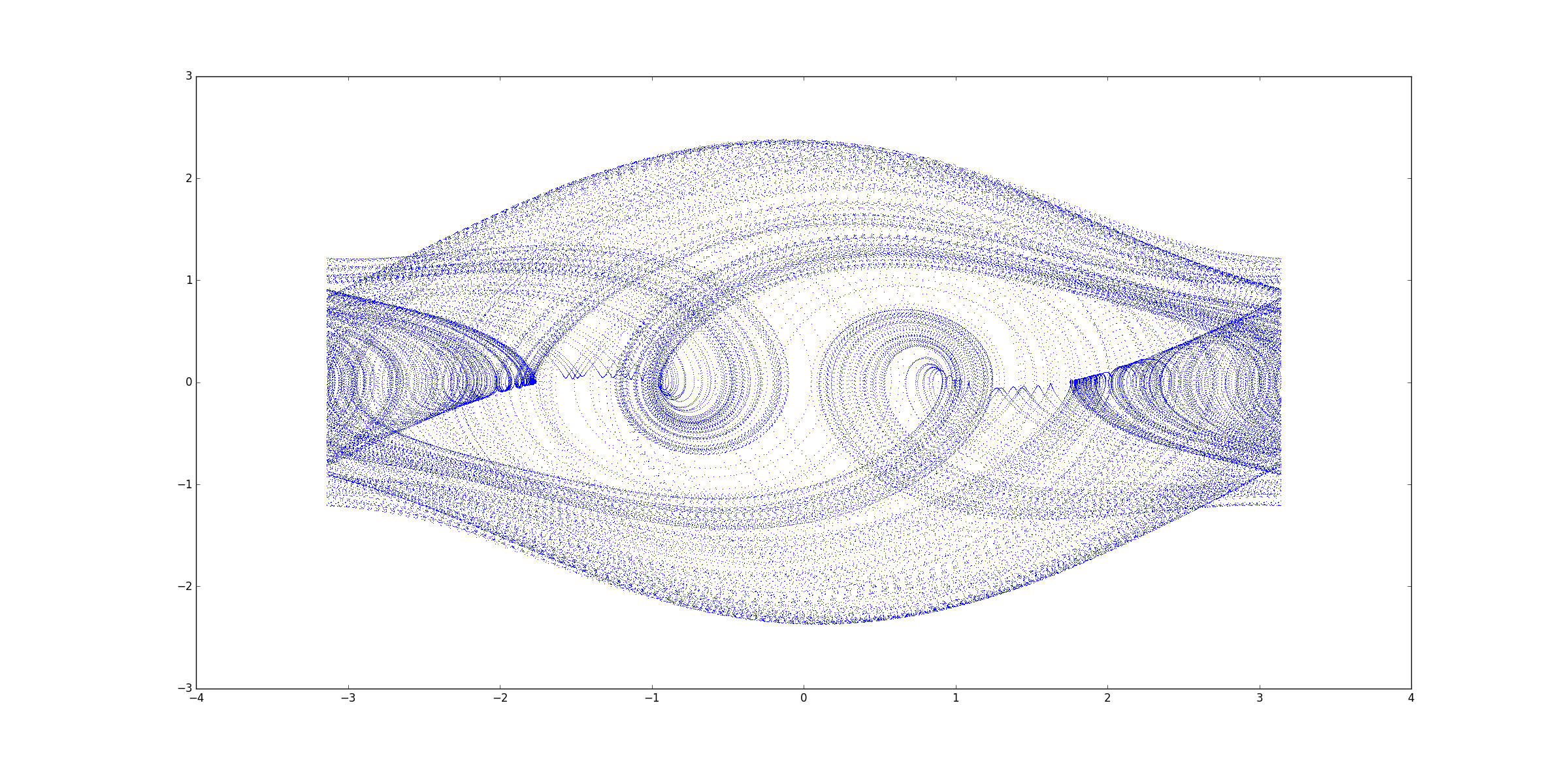
from pylab import *
import numpy as np
l=9.8
g=9.8
dt=0.04
q=0.5
F=1.2
D=2.0/3.0
class pendulum:
    def __init__(self,w,x,t):
        self.w=[w]
        self.x=[x]
        self.t=[t]
    def update(self):
        global g,dt,l
        current_w=self.w[-1]
        current_x=self.x[-1]
        current_t=self.t[-1]
        self.next_w=current_w-(g/l*np.sin(current_x)+q*current_w-F*sin(D*current_t))*dt
        self.next_x=current_x+self.next_w*dt
        self.next_t=current_t+dt
    def fire(self):
        while (self.t[-1]<=5000):
            self.update()
            if self.next_x>np.pi:self.next_x+=-2*np.pi
            else:
                if self.next_x<-np.pi:self.next_x+=2*np.pi
                else:self.next_x=self.next_x
            self.w.append(self.next_w)
            self.x.append(self.next_x)
            self.t.append(self.next_t)
        plot(self.x,self.w,',')
a=pendulum(0,3,0)
a.fire()
show()

图像如下图所示：

程序

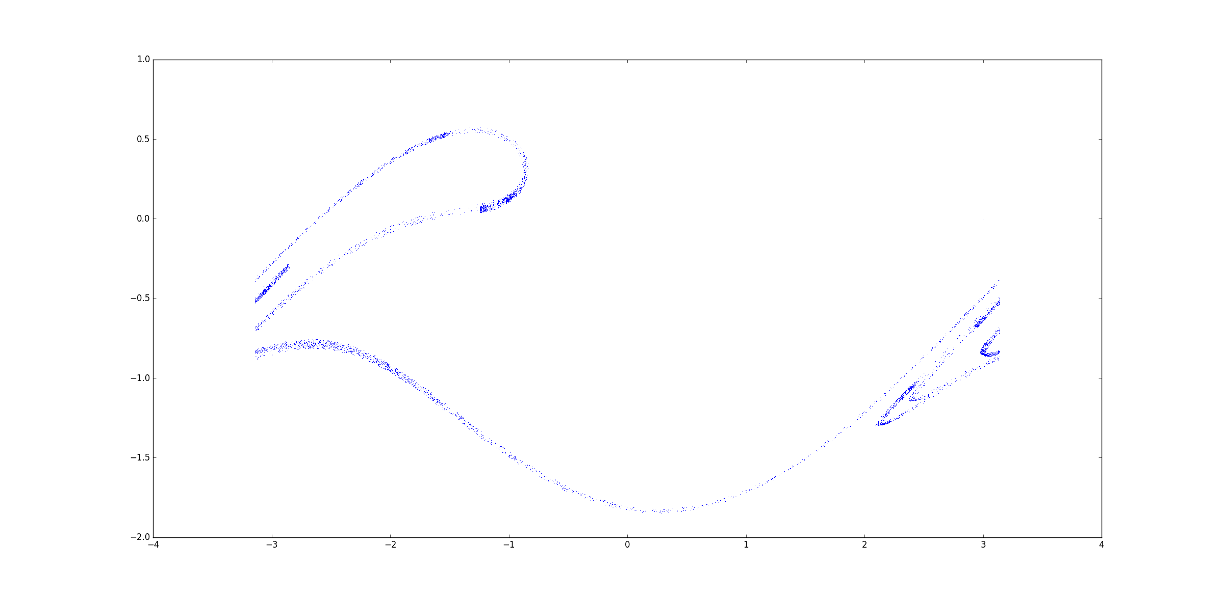
from pylab import *
import numpy as np
l=9.8
g=9.8
dt=0.04
q=0.5
F=1.2
D=2.0/3.0
class pendulum:
    def __init__(self,w,x,t):
        self.w=[w]
        self.x=[x]
        self.t=[t]
        self.chosen_w=[]
        self.chosen_x=[]
        self.chosen_t=[]
    def update(self):
        global g,dt,l
        current_w=self.w[-1]
        current_x=self.x[-1]
        current_t=self.t[-1]
        self.next_w=current_w-(g/l*np.sin(current_x)+q*current_w-F*sin(D*current_t))*dt
        self.next_x=current_x+self.next_w*dt
        self.next_t=current_t+dt
    def fire(self):
        while (self.t[-1]<=50000):
            self.update()
            if self.next_x>np.pi:self.next_x+=-2*np.pi
            else:
                if self.next_x<-np.pi:self.next_x+=2*np.pi
                else:self.next_x=self.next_x
            self.w.append(self.next_w)
            self.x.append(self.next_x)
            self.t.append(self.next_t)
            test=((self.t[-1]*D)%np.pi)/np.pi
            test2=self.t[-1]-int(self.t[-1]/np.pi)*np.pi
            #print test
            if (test<=0.01):
                if (test2<=1):
                    self.chosen_x.append(self.next_x)
                    self.chosen_w.append(self.next_w)
                    self.chosen_t.append(self.next_t)
                else:
                    pass
            else:
                pass
        plot(self.chosen_x,self.chosen_w,',')
        #plot(self.x,self.w,',',label='Chaos')
        #plot(self.chosen_x,self.chosen_w)
a=pendulum(0,3,0)
a.fire()
#legend(loc='best')
show()

• 当只选取 $t \approx 2\pi n/\Omega_D$ 相位的点时可得到如下图像。
  

结论

• 在非线性驱动力下可以产生混沌现象。