计算物理期末论文——Random Systems & Simple Ising Model

作者：夏海峰 学号：2013301020094

Abstract

• Random process is a collection of random variables representing the evolution of some system of random values over time. This is the probabilistic counterpart to a deterministic process (or deterministic system). Instead of describing a process which can only evolve in one way (as in the case, for example, of solutions of an ordinary differential equation), in a stochastic, or random process, there is some indeterminacy: even if the initial condition (or starting point) is known, there are several (often infinitely many) directions in which the process may evolve.
• This passage mainly discuss the fundamentalbehaviour of random system.And explore the relation between the random systems and the diffusion process.And do a little digging into the two_dimension Ising model.

KeyWords:

• Random Systems, Diffusion Process, 2-D Ising Model

Random Walk:

• At the begining ,we should discuss the most simple as well as the most fundamental example in random systems--the random walk of one dimension.
• The walker begins at the origion, and the first step is chosen at random at either to the right or the left,each with the probablitiety $\frac {1} {2}$.Then the next step was chosen, and agian the probablities for stepping left or right are both $\frac {1}{2}$ In a physical process such as the motion of a molecule in solution, the time between steps is approximately a constant, so the step number is roughly proportional to time. We will, therefore, often refer to the walker's position as a function of time.
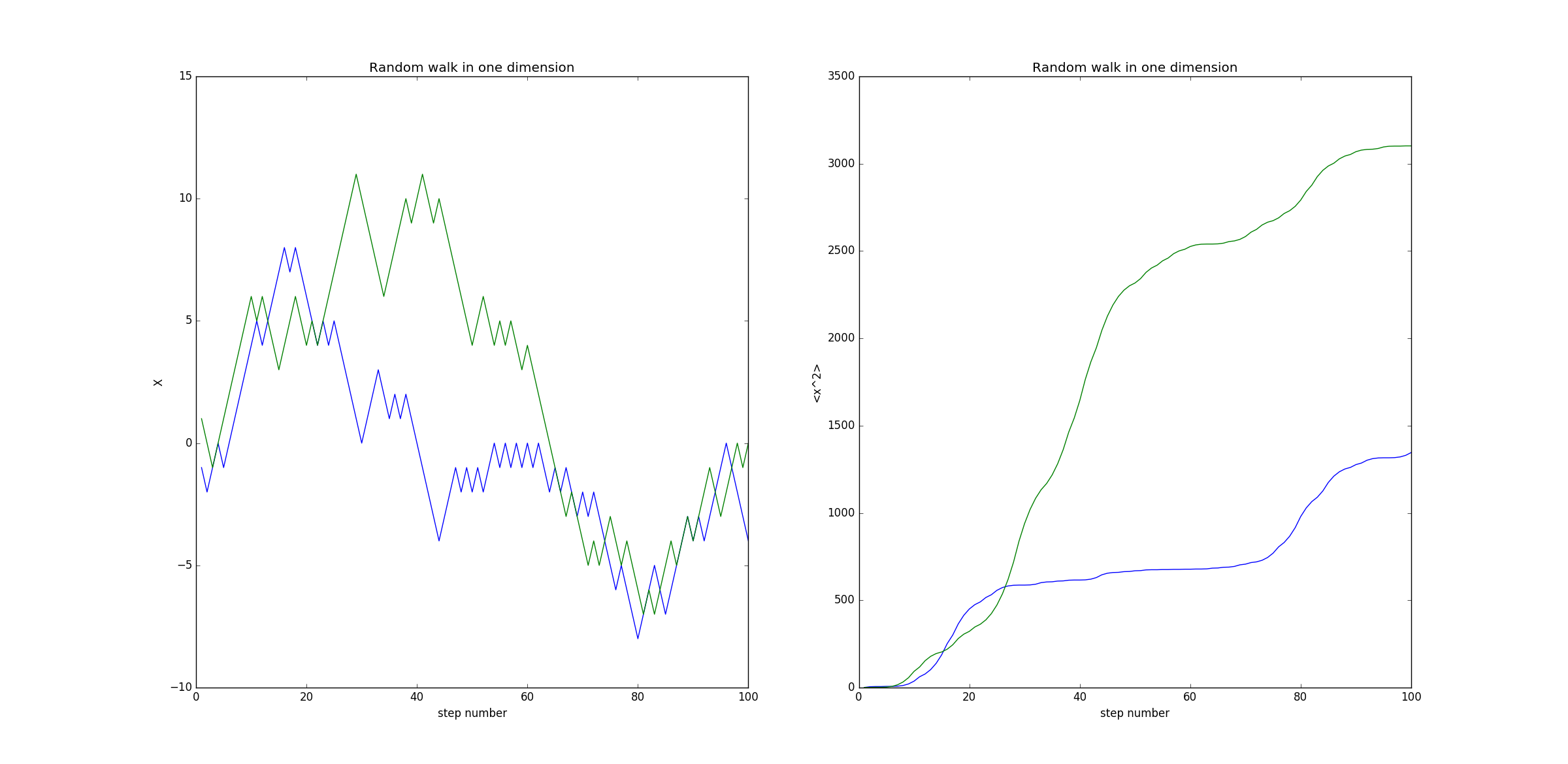
  Program

• The left part of the picture shows the path of the one dimension random walk.The right part shows the $x^2$ changes against steps.

• The reults are shown as blown:
  

• In a physical process such as the motion of a molecule in solution, the time between steps is approximately a constant, so the step number is roughly proportional to time. We will, therefore, often refer to the walker's position as a function of time.

• A more interesting and informative quantity is the average of the square of the displacement after n steps. Some results for this quantity are shown on the right in the above figure . We see that they are well described by a straight line, that is:
  

  $$<x^2>=2Dt------(1)$$
  where t is the time, which here is just equal to the step number; the factor D is known as the diffusion constant. 5 It is useful to compare this result with the behavior of a free particle, that is, one that is moving at a constant velocity and is not impeded by collisions with other particles. For such a particle we know that c=vt, so its distance from the origin (its starting point) grows linearly with time. A random walker behaves differently; according to (1) its root-mean-square
  distance from the origin grows only as $\sqrt {<x^2>} ~t^2$. Hence, a random walker escapes from the origin much more slowly than would a free particle.

• The motion of this sort can be expanded to the diffusion process.

From Random Systems to Diffusion process:

• Writing the position after n steps, as a sum of n sperate steps fives:
  $$x_n=\sum_{i=1}^n s_i$$
  $$x_n^2=\sum_{i=1}^n\left(\sum_{j=1}^ns_is_j\right)$$
• Since the steps are independent of each other, the terms $s_i$ $s_j$with $i\neq j$ will be $\pm 1$ with equal probability. If we average over a large number of separate walks this will leave only the terms with i j or s?. Thus we find :
  $$<x_n^2>=\sum_{i=}^ns_i^2$$

An alternative way to describe the same physics involves the density of particles,$\rho (y, z, t)$, which can be conveniently defined if the system contains a large number of particles (walkers). The idea, known as coarse graining, is to consider regions of space that are big enough to contain a large number of particles so that the density ( =mass/ volume) can be meaningfully defined. The density is then proportional to the probability per unit volume per unit time, denoted by z, t), to find a particle at (t, y, z) at time t. Thus, p and P obey the same equation. To find this equation, we focus back on an individual random walker. We assume that it is confined to take steps on a simple-cubic lattice, and that it makes one "walking step" each time step. P(i, j, k, n) is the probability to find the particle at the side (i, j, k) at time n. Since we are on a simple cubic lattice, there are 6 different nearest neighbor sites. If the walker is on one of these sites at time n — 1, there is a probability of 1/6 that it will then move to site (i, j, k) at time n. Hence, the total probability to arrive at (i, j, k) is :

$$P(i,j,k,n)=\frac {1}{6} \left[P(i+1,j,k,n-1)+P(i-1,j,k,n-1)+P(i,j+1,k,n-1)\\ +P(i,j-1,k,n-1)+P(i,j,k+1,n-1)+P(i,j,k-1,n-1)\right]$$
So:
$$P(i,j,k,n)-P(i,j,k,n-1)= \frac{1}{6} \lbrace P(i+1,j,k,n-1)-2P(i,j,k,n-1)+P(i-1,j,k,n-1)+ \\ P(i,j=1,k,n+1)-2P(i,j,k,n-1)+P(i,j-1,k,n-1)+\\ P(i,j,k+1,n-1)-2P(i,j,k,n-1)+P(i,j,k-1,n-1)\rbrace$$

Apart from a constant factor ($\frac {1}{\Delta t}$), the left side of this equation is just the finite difference approximation for the time derivative of P, while the right-hand side is proportional to a second order space derivative. This suggests taking the continuum limit, which leads to :

$$\frac {\partial P(x,y,z,t)} {\partial t}=D\nabla ^2P(x,y,z,t)-------------(2)$$
fusion equation. For ease of notation we will assume that p is a function of only one spatial dimension, x, although everyt,hing we do below can readily be extended to two or three dimensions. We can then write $\rho (x, t) = p(i\Delta x, n\Delta t) = p(i, n)$, so that the first index corresponds to space and the second to time. Converting (2) to one dimension yields :
$$\frac {\partial \rho}{\partial t}=D\frac {\partial^2 \rho}{\partial x^2}$$
$$\frac {\rho(i,n+1)- \rho(i,n)}{\Delta t}=\frac {\rho(i+1,n)- 2\rho(i,n)+\rho(i-1,n)}{\Delta t}$$
$$\rho(i,n+1)=\rho(i,n)+\frac {D \Delta t}{\left(\Delta x\right)^2}\left[\rho(i+1,n)+\rho(i-1,n)-2\rho(i,n)\right]$$

One Dimension Diffusion

Program

• From the figure above, we can see that the the displacement perfectly satisfy the Gaussian distribution.
• As the staps increases, the $\sigma$ becomes larger.
• Distribution function:
  $$\rho(x,t)=\frac {1}{\sigma}exp\left[{-\frac{x^2}{2\sigma ^2}}\right]$$
  $$\sigma=\sqrt {2Dt}$$

Cream in coffee

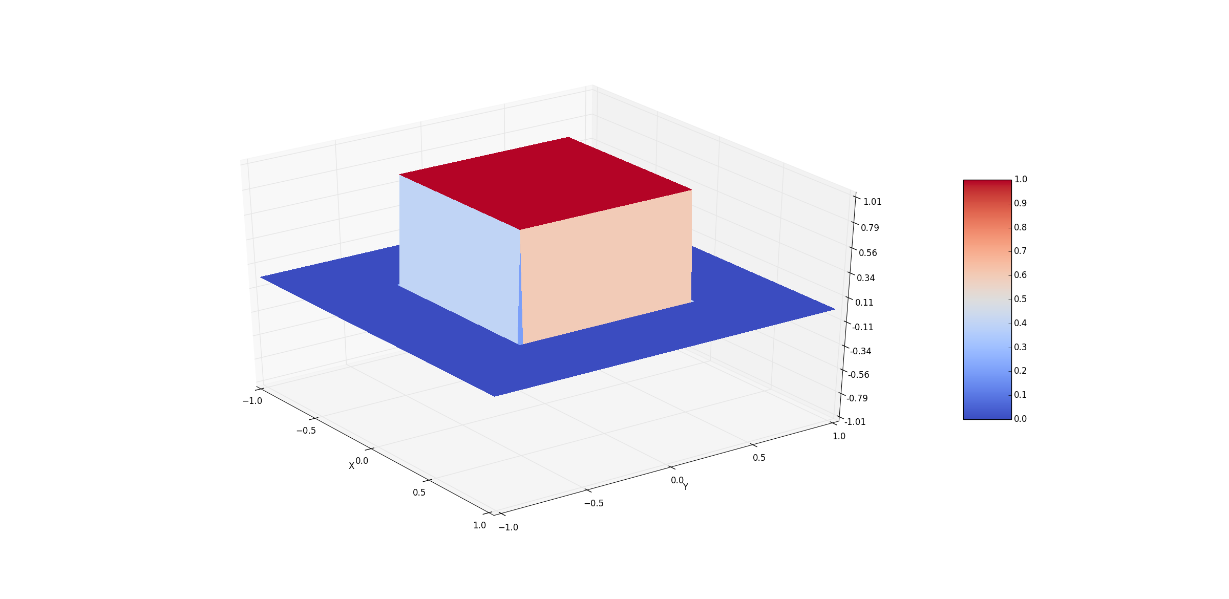
In this topic, we solve the problem which there is a cream in the center of the coffee. we exam the distriution of the cream as it merge with the coffee.

Methods:

• Diffusion equtaion evolve from random walk.
• $$P(i,j,n)=\frac {1}{4} \left[P(i+1,j,n-1)+P(i-1,j,n-1)+P(i,j+1,n-1) +P(i,j-1,n-1)\right]$$

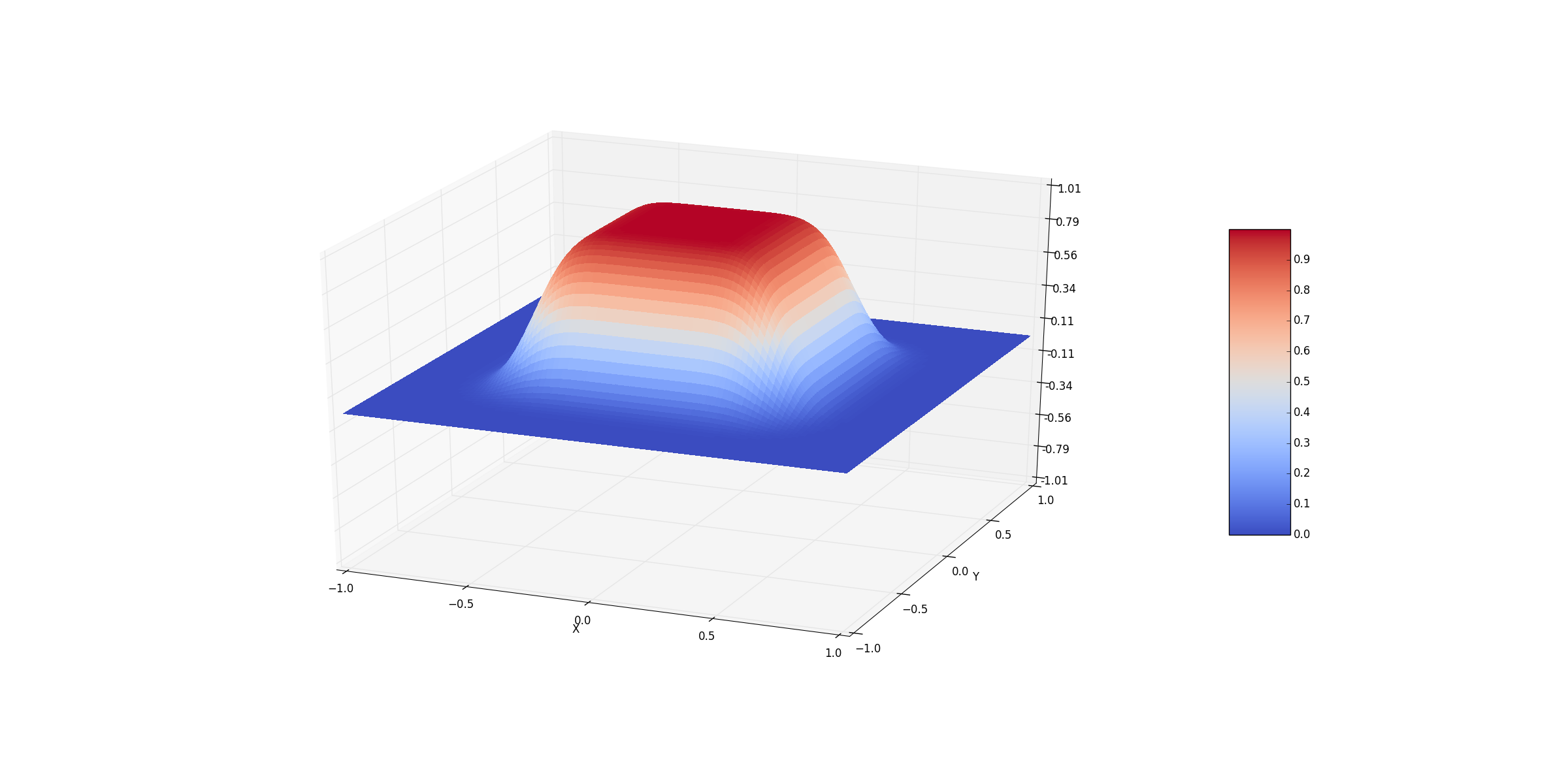
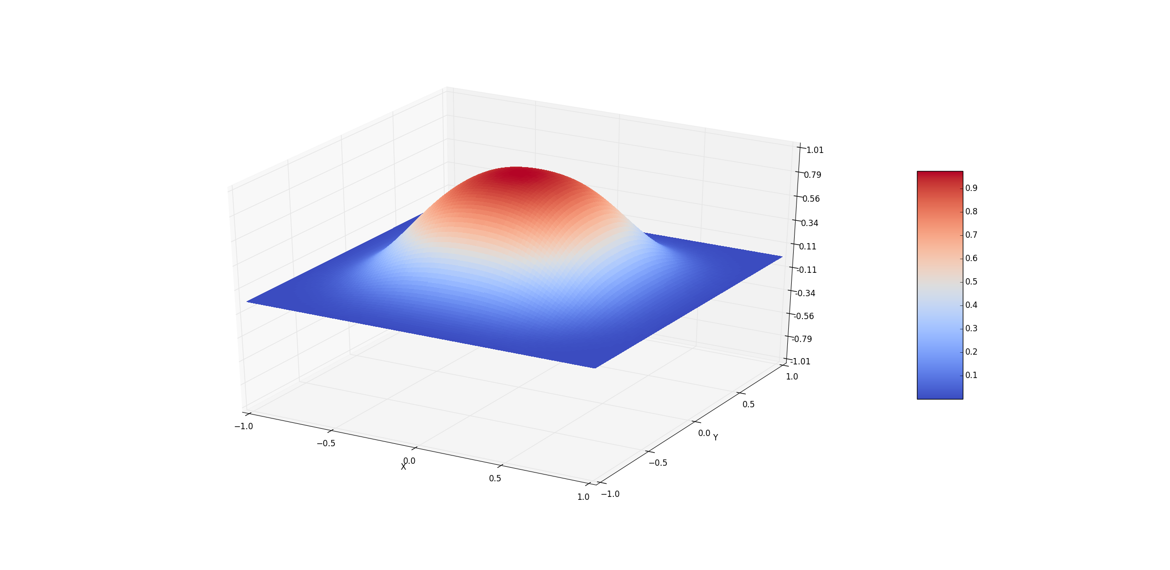
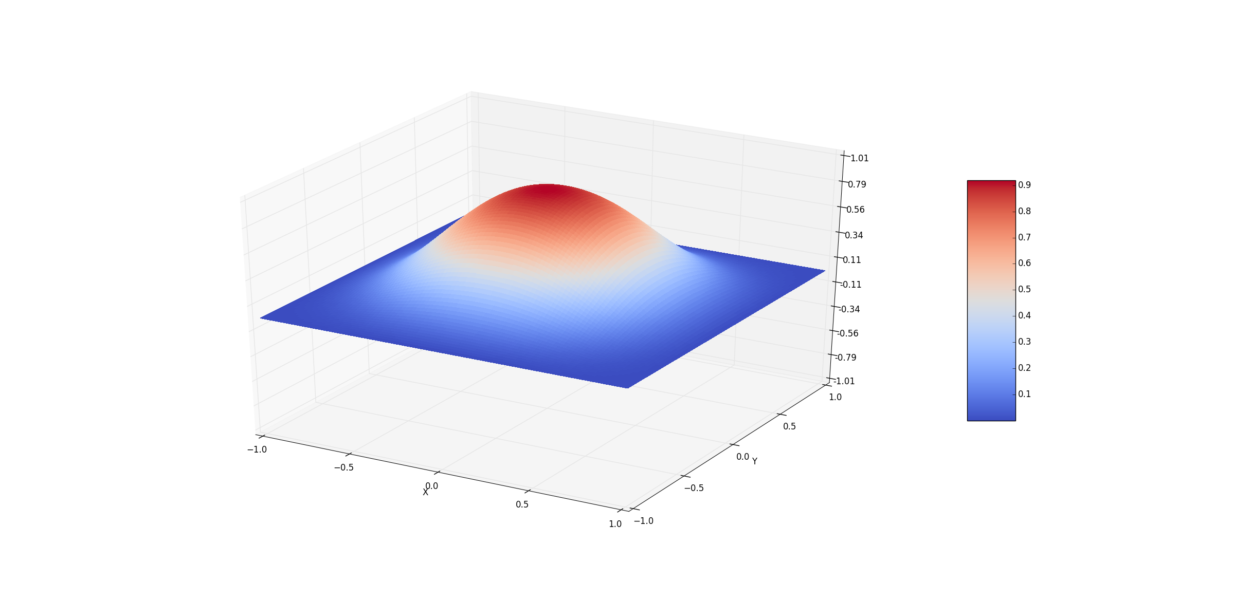
We can see how the cream melt in the folloing pictures:

Program

• At t=0(Initial):
  
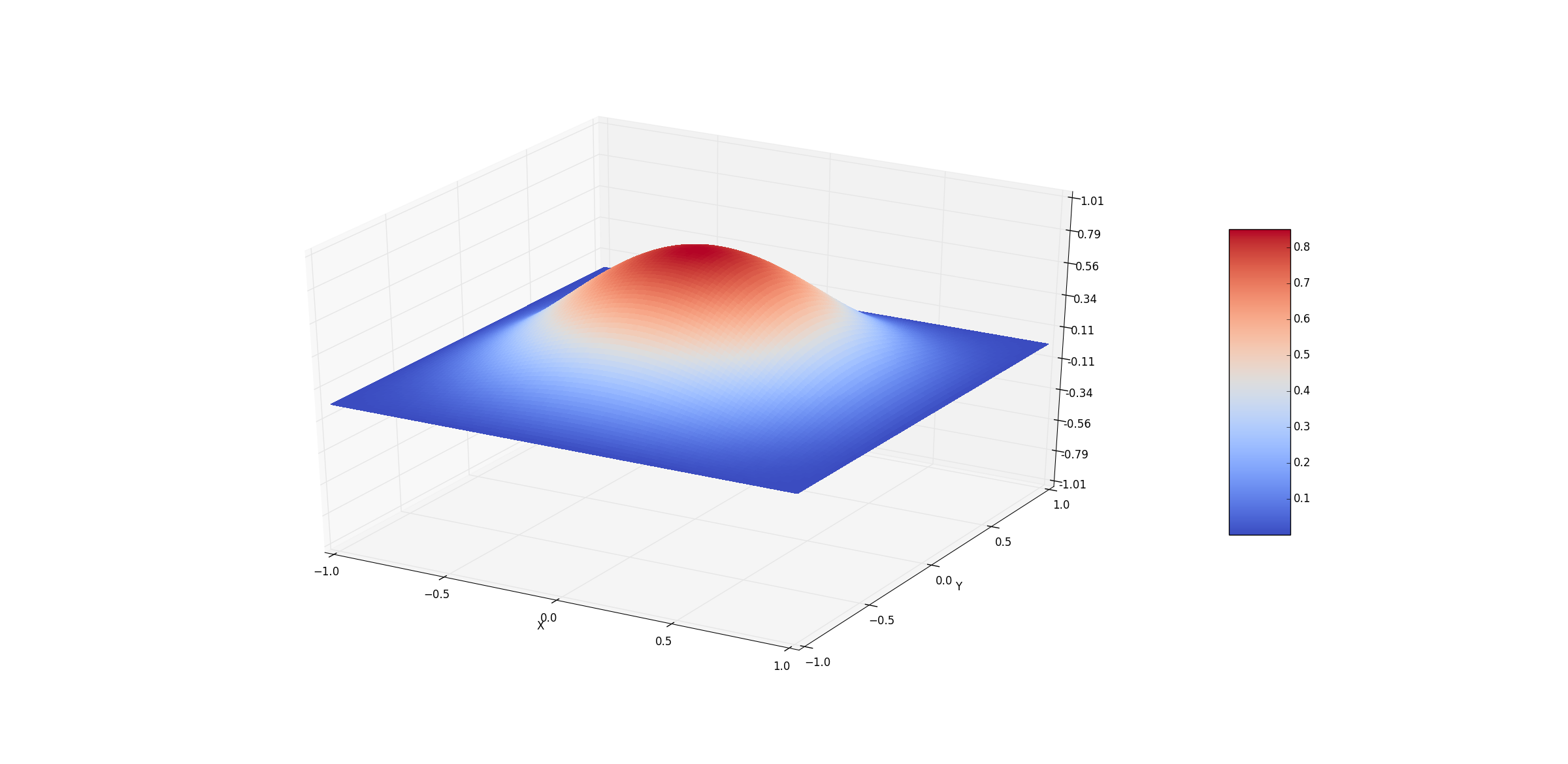
• At t=50 steps:
  
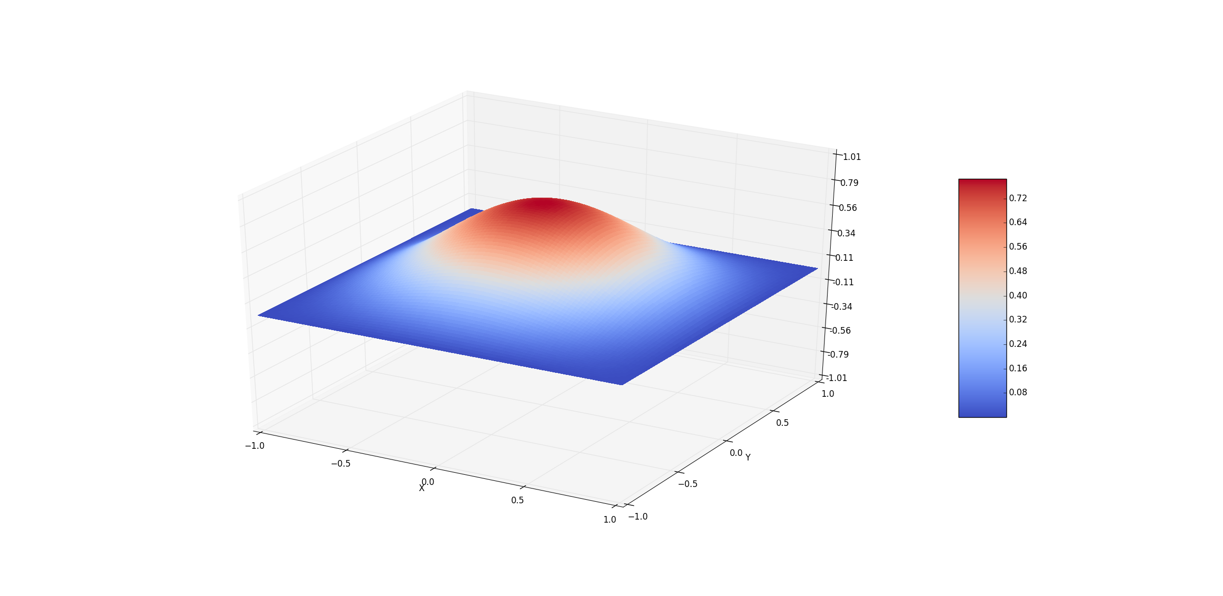
• At t= 200 steps:
  
• At t= 300 steps:
  
• At t= 400 steps:
  
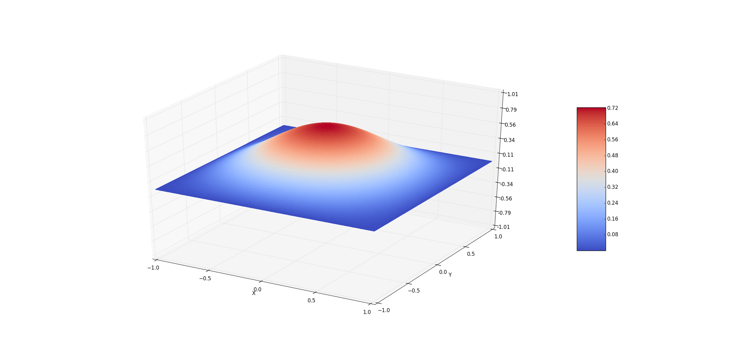
• At t= 500 steps:
  
• At t= 600 steps:
  
• At t=700 steps:
  
• At t= 1000 teps:
  
• At t= 1500 steps:
  
• At this point ,we can say that the cream has completely merged with the coffee.

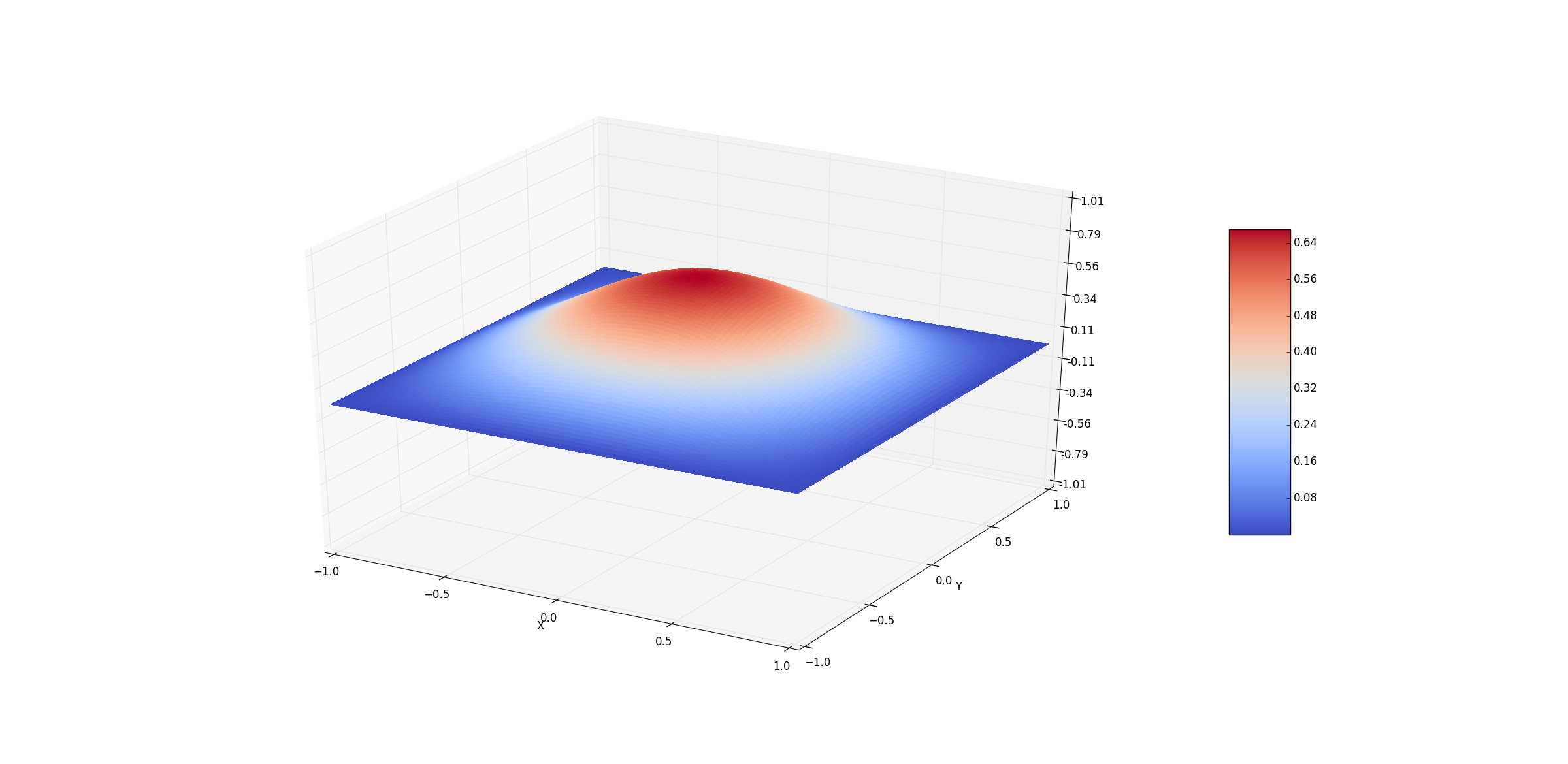
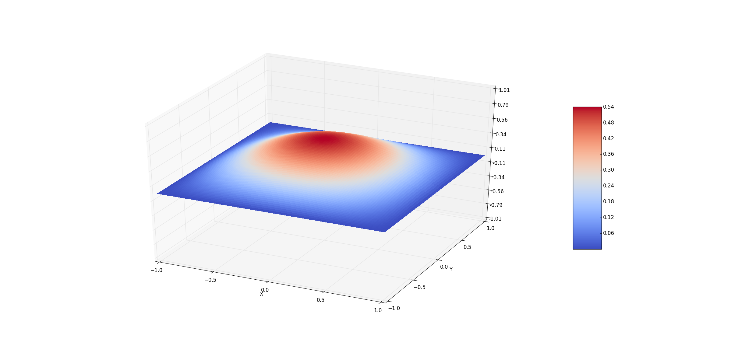
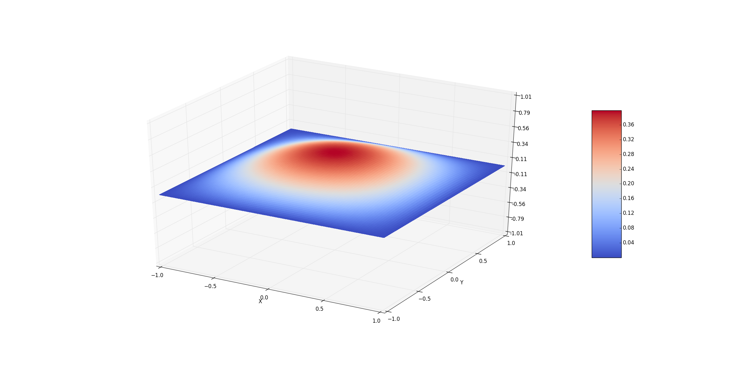
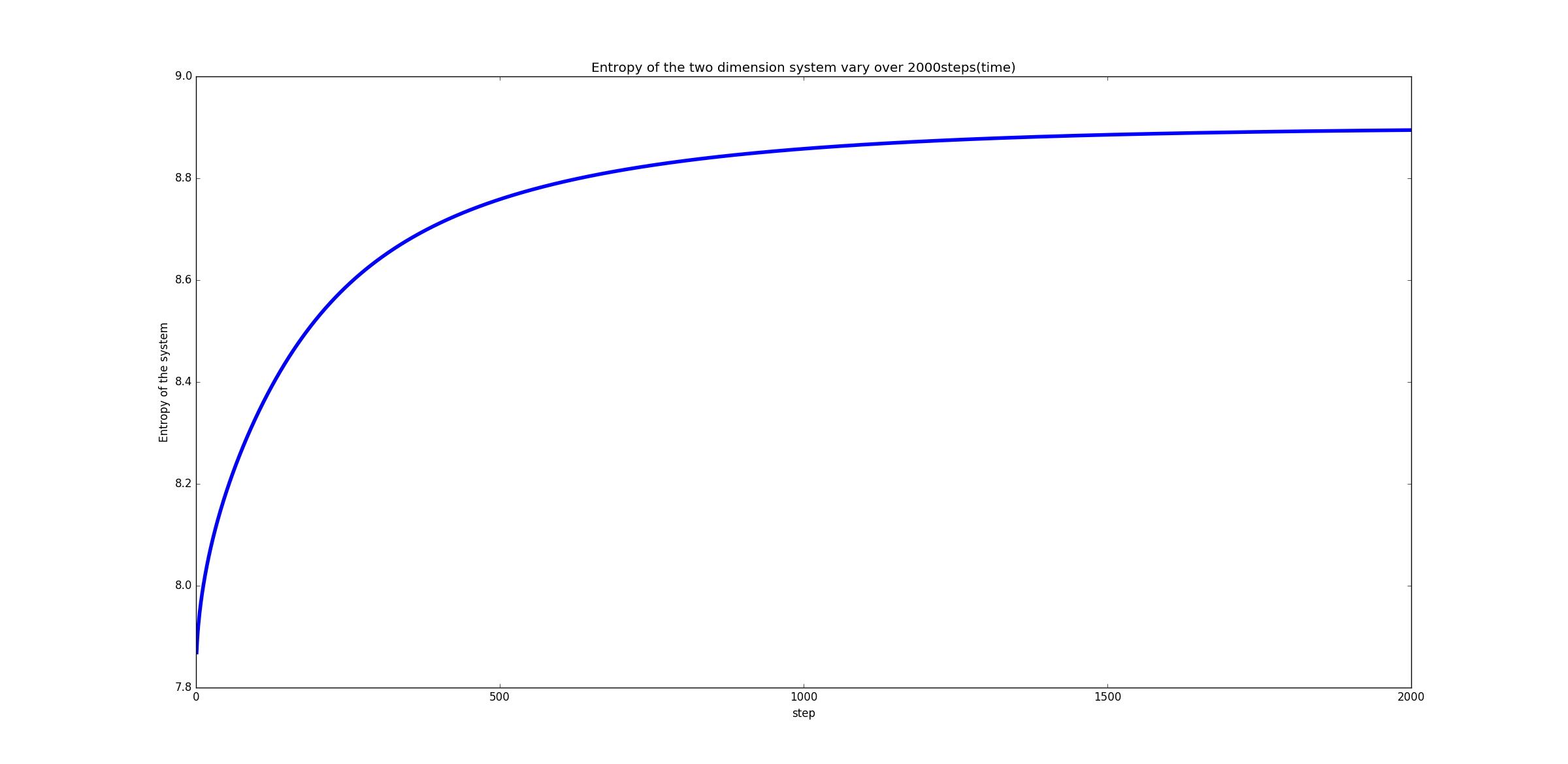
Two Dimension Diffusion Entropy

Calculating method:

• Statistical definition of entropy:
  $$S= -\sum_{i}^n P_i\ln {P_i}$$
  Program
  

Isning Model

Therotical Fundation:

• Ising Model:
  (1)Basic Introduction:
  The Ising model, named after the physicist Ernst Ising, is a mathematical model of ferromagnetism in statistical mechanics. The model consists of discrete variables that represent magnetic dipole moments of atomic spins that can be in one of two states (+1 or −1). The spins are arranged in a graph, usually a lattice, allowing each spin to interact with its neighbors. The model allows the identification of phase transitions, as a simplified model of reality. The two-dimensional square-lattice Ising model is one of the simplest statistical models to show a phase transition.

The Ising model was invented by the physicist Wilhelm Lenz (1920), who gave it as a problem to his student Ernst Ising. The one-dimensional Ising model has no phase transition and was solved by Ising (1925) himself in his 1924 thesis. The two-dimensional square lattice Ising model is much harder, and was given an analytic description much later, by Lars Onsager (1944). It is usually solved by a transfer-matrix method, although there exist different approaches, more related to quantum field theory.

In dimensions greater than four, the phase transition of the Ising model is described by mean field theory.
(2)Basic Theory:
The energy of the system is:

$$E=-J \sum_{<ij>}{s_i s_j}$$
The sum is over all pairs of nearest neighbour spin $<ij>$.
It is a fundamental result, of statistical mechanics that for a system in equilibrium with a heat bath, the probability of finding the system in any particular state is proportional to the Boltzmann factor :
$$P_{\alpha} =e^{E_{\alpha}/k_BT}$$
The measure magnetization of the system will then be:
$$M=\sum_{\alpha}{M_{\alpha}P_{\alpha}}$$
(2)Calculation Methods:

• Monte Carlo algorithim for the Ising model on an L$\times$L square lattice
  (1)Set the desired T and H
  (2)Initialize the spin $s_i$ $(i=1,2, {\ldots} ,L^2)$
  (3)Perform 1000 times Monte Carlo sweeps through lattice.

• For every sweep,loop through the L rows of the lattice
  (1) Flip the spin, and calculate the energy before and after the operation.
  

  $$E_{Flip}=E_{former}-E_{later}$$
  (2)If $E_{Flip} <0$,then the spin remian flipped (surive in this operation)
  (3)If $E_{Flip} <0$, generate an random number between 0 and 1,named it r, and
  compare it to $\exp ({E_{Flip}/K_B T})$
  If $r \leq \exp ({E_{Flip}/K_B T})$ , then the spin remian flipped (surive in this operation).
  Else, the spin should be flipped back.
  (4)Calculate the energy and magnetization of the system.

• Energy & Magnetization versus tempature
  Program(This program takes over six minutes to be finished! Testing CPU：Core i7-4710HQ @2.5GHz-3.5GHz）
  
  
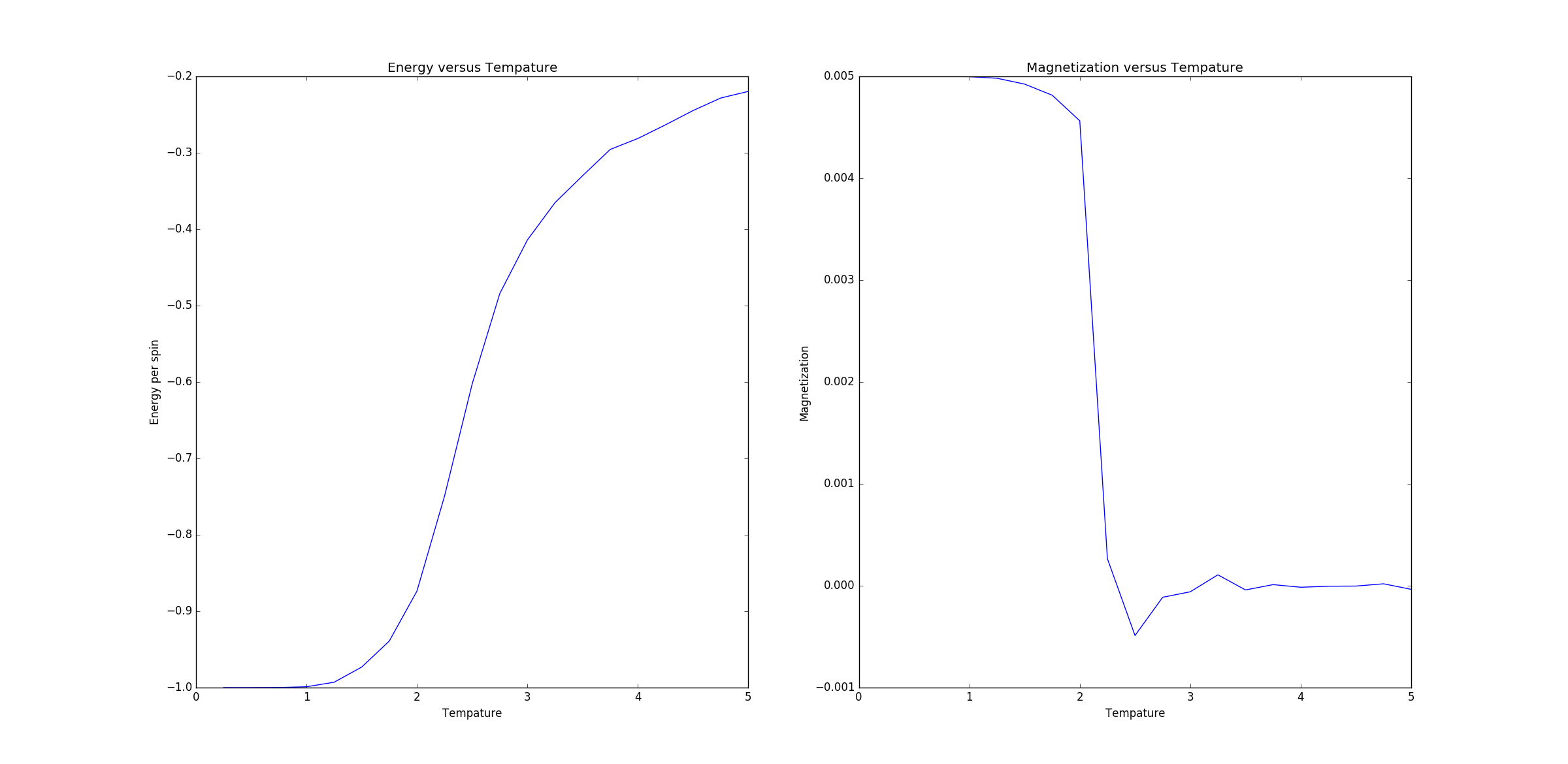
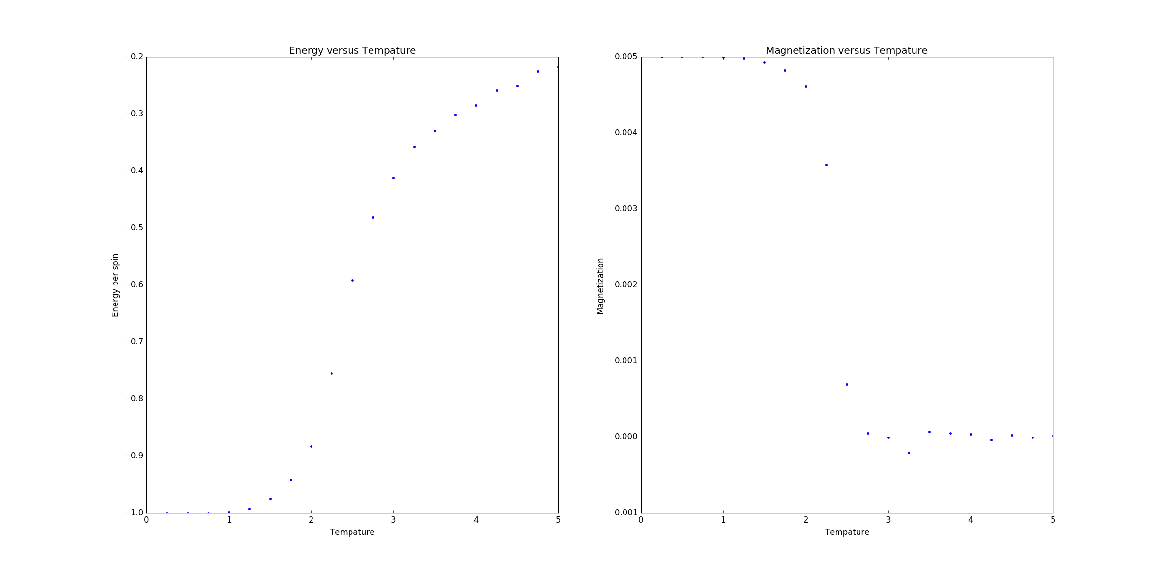
  We can see from the picture that the critical tempature is somewhere between 2K and 3K.

• Here is the picture of the magnetization of the system, with more tempature calculated between 2k and 3k.
  
• Magnetization versus times(steps)
  Program
  

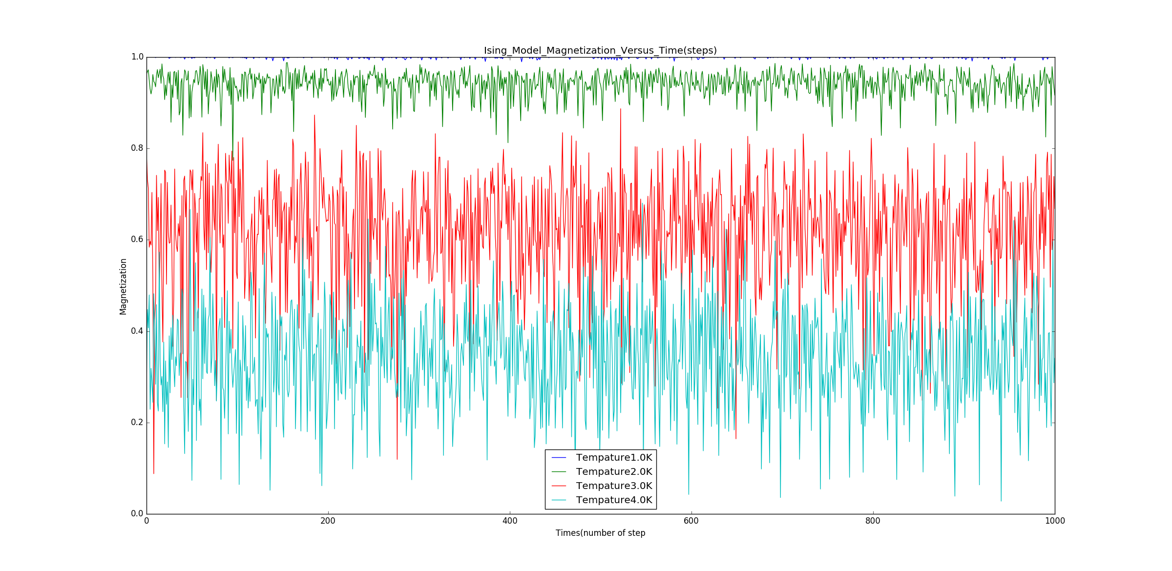
We can see that ,during the process of Monte-Carlo simulation,the magnetization of the system changes sharply,but in different tempature regions,the magnetization varies accordingly. With tempature increasing,the magnetization ,on sacle, decreases.

Conclusion

• The Ising model and the random system are closely related.
• The systems(random systems) always have the tendency to the states that have more entropy.
• The magnetization of Ising model system is dependent of tempature.
• There exists a critical tempature that there is phase transition in Ising model system, and that critical tempature is somewhere between 1 K and 2 K.

Reference

• Computational Physics, 2nd Edition,Nicholas J. Giordano & Hisao Nakanishi, 7th Chapter-Random systems
• Computational Physics, 2nd Edition,Nicholas J. Giordano & Hisao Nakanishi, 8th Chapter-
  Statistical Mechnaics, Phase Transition, and The Ising Model.