@zy-0815
2016-10-30T14:47:51.000000Z
字数 5541
阅读 1802
张梓桐计算物理第七次作业
1.Problem
3.12,3.13,3.14
2.Abstract
Having dicussed the Euler method in calculating projectile movement of a cannon shell,in the passage,we are going to talk about the Euler-Cromer method of the better calculation of oscillatory under damped and external force.
3.Background
Now we start to figure out the movement rule of a damped and forced pendulum.With the basic knowledge of Newtoon second law and the definition of , we have the following equation:
where is the module of the external force with unit,and is the frequency of external force,also with unit.
Here we introduce the variables to transfer the secdonary differential equation into firs-order differential equation:
Now we rewrite the physics formula into precodes,notcing the Euler-Cromer method,rather than Euler method,which will lead to a divergence in the infinity.
For each time step ,calculate and at time step .
If is out of the ,add or substract to keep it in this range.
Repeat for the deisred number of time steps.
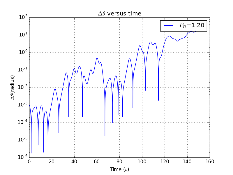
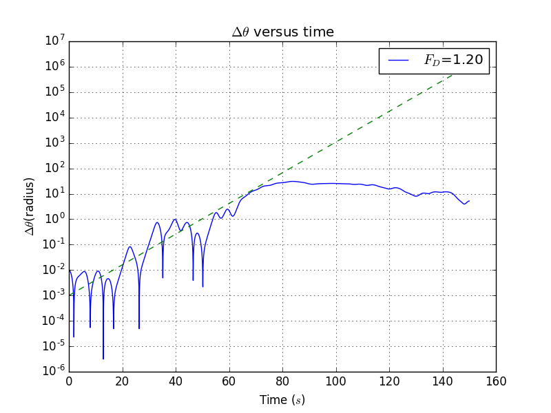
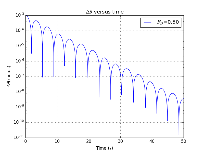
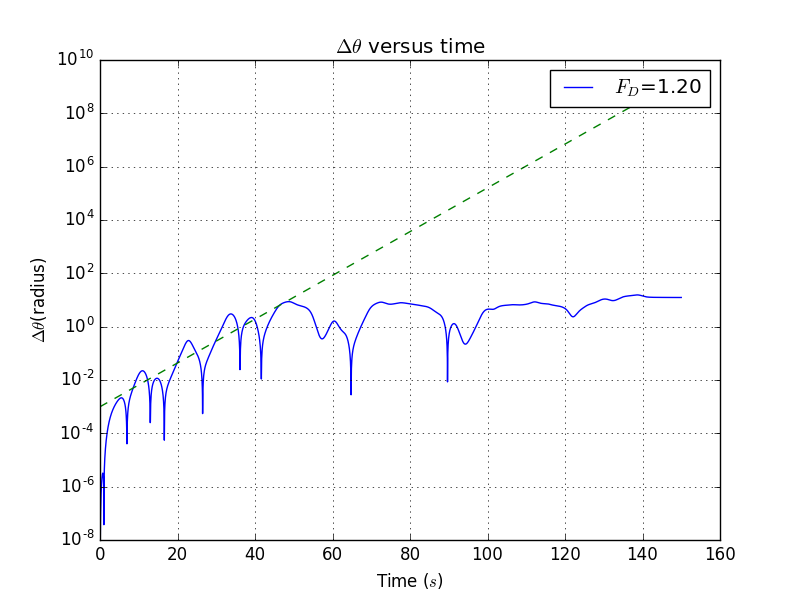
In problem 3.13 and 3.14,we are asked to calculate the and compare the behacior of two,nearly identical pendulums.And we are going to draw a ' versus time' plot.
3.Main body
3.1 Solution to 3.13,3.14
import mathimport pylab as plclass oscillatory_motion():def __init__(self):intial_theta=0.2intial_w=0time_of_duration=150self.theta=[intial_theta]self.t=[0]self.w=[intial_w]self.dt=0.04self.q=0.5self.F_D=1.2self.w_D=0.6666667self.nsteps = int(time_of_duration // self.dt + 1)self.w2=[intial_w]self.theta2=[intial_theta+0.001]self.a=[abs(self.theta[0]-self.theta2[0])]def run(self):for i in range(self.nsteps):#set an arbitrary time limit of the plottmp_w=self.w[i]-(math.sin(self.theta[i])+self.q*self.w[i]-self.F_D*math.sin(self.w_D*self.t[i]))*self.dtself.w.append(tmp_w)tmp_theta=self.theta[i]+self.w[i+1]*self.dtself.theta.append(tmp_theta)# while self.theta[-1]>1*math.pi:# self.theta[-1]=self.theta[-1]-2*math.pi#while self.theta[-1]<-1*math.pi:# self.theta[-1]=self.theta[-1]+2*math.pitmp_w2=self.w2[i]-(math.sin(self.theta2[i])+self.q*self.w2[i]-self.F_D*math.sin(self.w_D*self.t[i]))*self.dtself.w2.append(tmp_w2)tmp_theta2=self.theta2[i]+self.w2[i+1]*self.dtself.theta2.append(tmp_theta2)# while self.theta2[-1]>1*math.pi:# self.theta2[-1]=self.theta[-1]-2*math.pi#while self.theta2[-1]<-1*math.pi:# self.theta2[-1]=self.theta2[-1]+2*math.piself.t.append(self.t[i]+self.dt)self.a.append(abs(self.theta[i+1]-self.theta2[i+1]))def show(self):pl.semilogy(self.t, self.a,label='$F_{D}$=%.2f'%self.F_D)pl.xlabel('Time ($s$)')pl.ylabel('$\Delta \\theta $(radius)')pl.title('$\Delta \\theta $ versus time')pl.legend(loc='upper right',frameon = True)pl.grid(True)pl.show()a=oscillatory_motion()a.run()a.show()
3.2 Solution to 3.12
import mathimport pylab as plclass oscillatory_motion():def __init__(self):intial_theta=0.2intial_w=0time_of_duration=10000self.theta=[intial_theta]self.t=[0]self.w=[intial_w]self.dt=0.01self.q=0.5self.F_D=1.2self.w_D=0.6666667self.nsteps = int(time_of_duration // self.dt + 1)self.tmp_w=[0]self.tmp_theta=[0]def run(self):for i in range(self.nsteps):#set an arbitrary time limit of the plottmp_w=self.w[i]-(math.sin(self.theta[i])+self.q*self.w[i]-self.F_D*math.sin(self.w_D*self.t[i]))*self.dtself.w.append(tmp_w)tmp_theta=self.theta[i]+self.w[i+1]*self.dtself.theta.append(tmp_theta)while self.theta[-1]>1*math.pi:self.theta[-1]=self.theta[-1]-2*math.piwhile self.theta[-1]<-1*math.pi:self.theta[-1]=self.theta[-1]+2*math.piself.t.append(self.t[i]+self.dt)for i in range(self.nsteps):if self.t[i]%(2*math.pi/self.w_D)<0.01:self.tmp_w.append(self.w[i])self.tmp_theta.append(self.theta[i])def show(self):pl.plot(self.tmp_theta, self.tmp_w,'.',label='$F_{D}$=%.2f'%self.F_D)pl.xlabel('$\\theta$ (radians)')pl.ylabel('$w$(radius/s)')pl.title('$w$ versus $\\theta$')pl.legend(loc='upper right',frameon = True)pl.grid(True)pl.show()a=oscillatory_motion()a.run()a.show()
4.Result
4.1 Result with different intial angle.
Here the parameters are , , , ,
Here are the expoential simulation plot:()
Here the parameters are , , , ,
Here are the expoential simulation plot:()
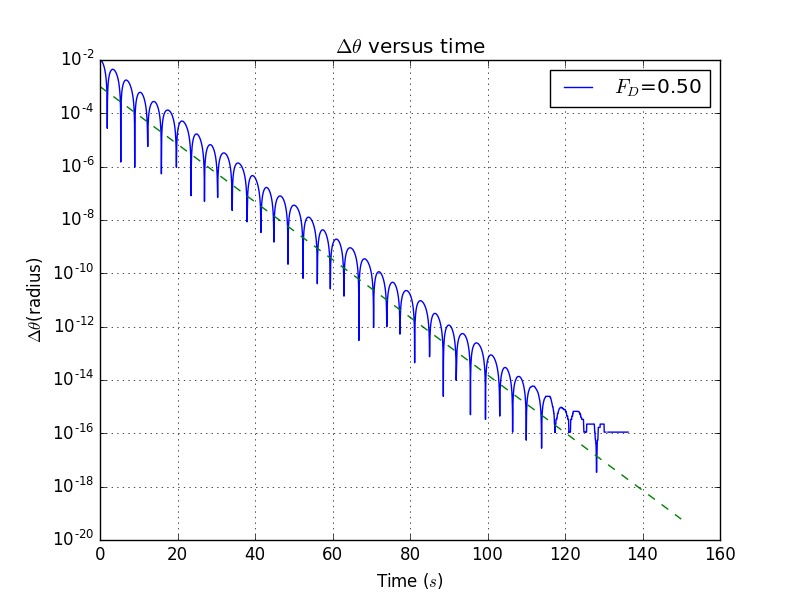
Here are the photos with different of ' versus time' plots
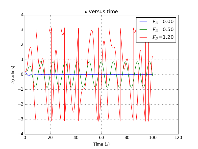
Here are the photos with different of ' versus time' plots

4.2 Result with different damping factors
Here the parameters are , , , ,
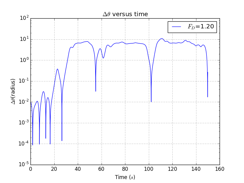
Simulation:()
Here the parameters are , , , ,
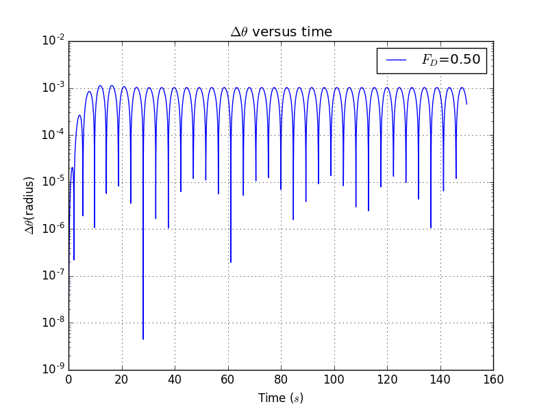
Simulation plot():

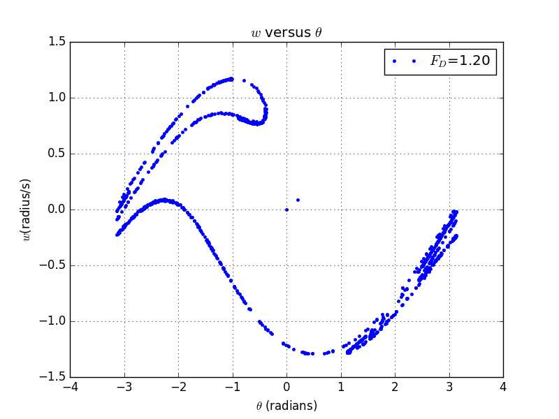
4.3 Result with 3.12
Here the parameters are , , , ,,time duration =10000.This is a plot corresponding to a maximum of the frive force.
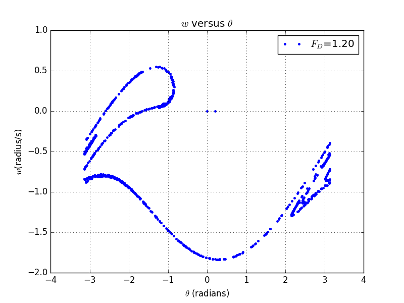
This is a plot corresponding to a phase of the frive force.
6.Ackanowledgement
After my dicsussion,here is one thing that I want to stress.Withoud the attention of the calculation of computer,I ignore the difference of fraction and decimal,which led to a serious and confusing problem,that is, I mistakely took as 0.67.This problem leads to a zero result with my external force and out of which I had struggled almost two hours to figure it out.And I want to thanks to Yukang,who found its out but he didn't know why at first and finally told by Wang shixing.Thanks to both of them.
7.Refernece
1.Yu kang for his help in
2.Matplotilb
3.<< How to think like a computer scientist>>
