张梓桐计算物理第十次作业

1 Problem

4.10

2 Abstract

From the prsent chapter we will consider several problems that arises in the study of plantery motion.We firstly begin with the simplest situation where a sun and a single planet get moved with interaction.We investigate a few of the properities of this model solar system.The very firts thing that we would like to investigate is the Kepler' laws of motion.Additionally,the inverse-square law and the stability of plantery orbits will be discussed.In the end,we will study the precession of the perihelion of Mercury.

3 Background

3.1 Kepler's Laws

There is only one planet which we will refer to as earth,which is in the orbit of sun.It's also the so-called two-body problem.According to Newton's law of gravitation the magnitude of this force is given by

$$\begin{eqnarray*} F_G=\frac{GM_S M_E}{r^2} \end{eqnarray*}$$
What we aimed to do is to calculate the position of earth as a function of time.From the Newton's Laws of motion we obtain:
$$\begin{eqnarray*} \frac{d^2x}{dt^2}=\frac{F_{G,x}}{M_E}\quad\frac{d^2y}{dt^2}=\frac{F_{G,y}}{M_E} \end{eqnarray*}$$
Note that :
$$\begin{eqnarray*} cos\theta=\frac{x}{r}\quad sin\theta=\frac{y}{r} \end{eqnarray*}$$
We obtain:
$$\begin{eqnarray*} \frac{dv_x}{dt}=-\frac{GM_S x}{r^3} \quad \frac{dx}{dt}=v_x \end{eqnarray*}$$
$$\begin{eqnarray*} \frac{dv_y}{dt}=-\frac{GM_S y}{r^3} \quad \frac{dy}{dt}=v_y \end{eqnarray*}$$
Worth mentioning,the selection of $SI$ is of great importance.We here chooe the distance $r$ between earth and sun to be $1AU$.And the time unit to be $1yr$.Thus we obtain:
$$\begin{eqnarray*} GM_S=v^2r=4\pi^{2}(AU^3/yr^2) \end{eqnarray*}$$ .
We next convert the equations of motion into difference equations in preparation of contructing a computational solution:

At each time step $i$ calculate the position $(x,y)$ and the velocity $(v_x,v_y)$ for time step $i+1$ using the Euler-Cromer method.

• Calculate the distance $r_i$ from the sun:$r_i=(x_i^2+y_i^2)^{1/2}$.

• Compute $v_{x,i+1}=v_{x,i}-\frac{4\pi^{2}x_i}{r_i^{3}}\Delta t$ and $v_{y,i+1}=v_{y,i}-\frac{4\pi^{2}y_i}{r_i^{3}}\Delta t$.

• The Euler-Cromer step:calculate $x_{i+1}=x_i+v_{x,i+1}\Delta t$,$y_{i+1}=y_i+v_{y,i+1}\Delta t$.

• Record the new position or plot as it becomes availiable.

• Repeat for desired number of time steps.
  

  Illustration of Kepler's three laws with two planetary orbits.
  (1) The orbits are ellipses, with focal points $ƒ_1$ and $ƒ_2$ for the first planet and $ƒ_1$ and $ƒ_3$ for the second planet. The Sun is placed in focal point $ƒ_1$.
  (2) The two shaded sectors A1 and A2 have the same surface area and the time for planet 1 to cover segment A1 is equal to the time to cover segment A2.
  (3) The total orbit times for planet 1 and planet 2 have a ratio $a_1^{3/2}$ : $a_2^{3/2}$.

3.2 The inverse-square law and the stability of plantery orbits

Here we are going to begin with a quick review of a few analytical results concerning the trajectory of a body in a solar system assumed to contain only the Sun and the body.

Kepler's laws tell us that the orientation of such an orbit does not change with time.More precisely,if we have a solar system consisting of a sun and one planet,and that one planet,and that follows an elliptical orbit,it is predicted that the orientation of the axes of the ellipse does not change with time.

Now let us suppose that the force law deviates slightly from an inverse-square dependence.To be specific,suppose that the gravational force is of the form:

$$\begin{eqnarray*} F_G=\frac{GM_S M_E}{r^\beta} \end{eqnarray*}$$
On the condition of $\beta=2$ we obtain the inverse-square law.Nevertheless we also want to conisder the motion of our planet for values of $\beta$ not equal to 2.The elleptical orbits with this force law can be simulated with the planteary motion program given above by simply changing the exponent of $r$ in the equations for the velocity.

3.3 The precession of the perihelion of Mercury

Perhaps you may be impressed with a simple superficial situation that all the precise movemet of planet can be calclated by the previous program precisely.Nevertheless,there are deviations from these laws.These deviations come from a number of sources,including the effects of the planets on each other.It turns out that this is a problem for which very few exact results are known.

Of most importance is the precession of the perihelion of Mercury.The planets whose orbits deviate the most from circular are Mercury and Pluto.

For Mercury it was known by the early part of the 19th century that the oreientation of the axes of the ellipse that describes its orbit rotate with time.

Discrepancies between the observed perihelion precession rate of the planet Mercury and that predicted by classical mechanics were prominent among the forms of experimental evidence leading to the acceptance of Einstein's Theory of Relativity (in particular, his General Theory of Relativity), which accurately predicted the anomalies. Deviating from Newton's law, Einstein's theory of gravitation predicts an extra term of $\frac{A}{r^4}$, which accurately gives the observed excess turning rate of 43″ every 100 years.

This was one of the first triumph of the theory of relativity.
The precession due to general relativity can be calculated analytically,allthough to do si is fairly complicated.However,it's actually very strightforward to deal with this problem computationally.
All we have to do is simulate the orbital motion using the force law predicted by the general relativity and measure the rate of precession of the orbit.

$$\begin{eqnarray*} F_G\approx\frac{GM_S M_M}{r^2}(1+\frac{\alpha}{r^2}) \end{eqnarray*}$$

4 Main Body

Source code

5 Discussion

5.1 Basic proprities

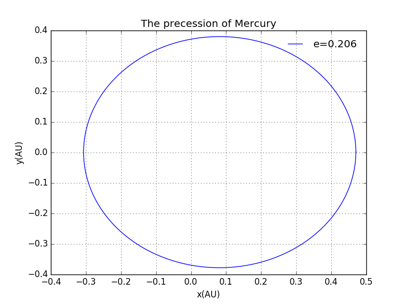
Here we plot the general movement trajectory of a Mercury of 1 period.Consequently,no further precession can be seen as a result of one period only.

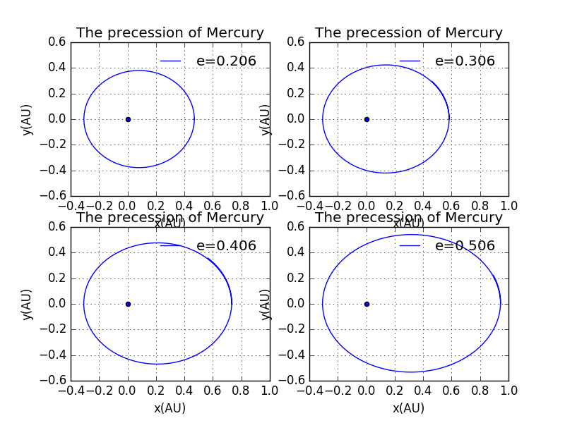
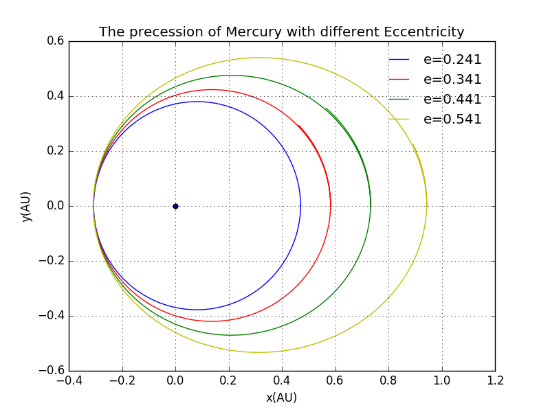
Next ,let us see the behave of the Mercury of different eccentricity.We shall see with bigger eccentricity,the trajecory becomes more elletical,as suggested by the definition of eccentricity.

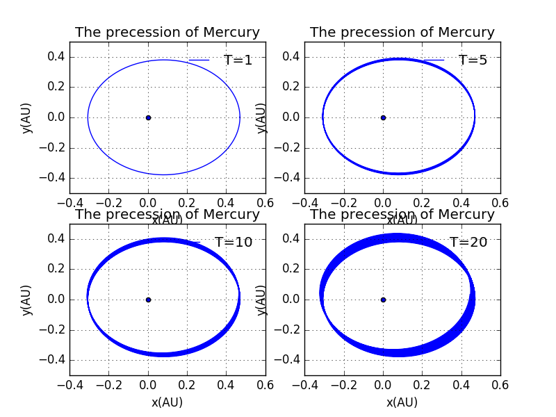
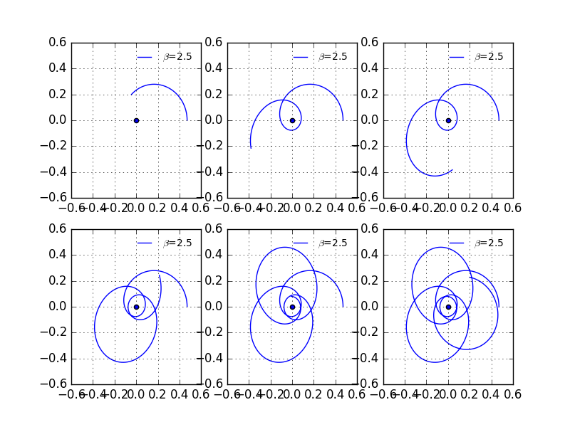
Here we shall the progress of the precession of Mercury but giving differnet duration of time.It's evidently that the trajectory is gradually turnning the orientatino as predicted.

Details

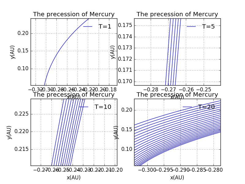
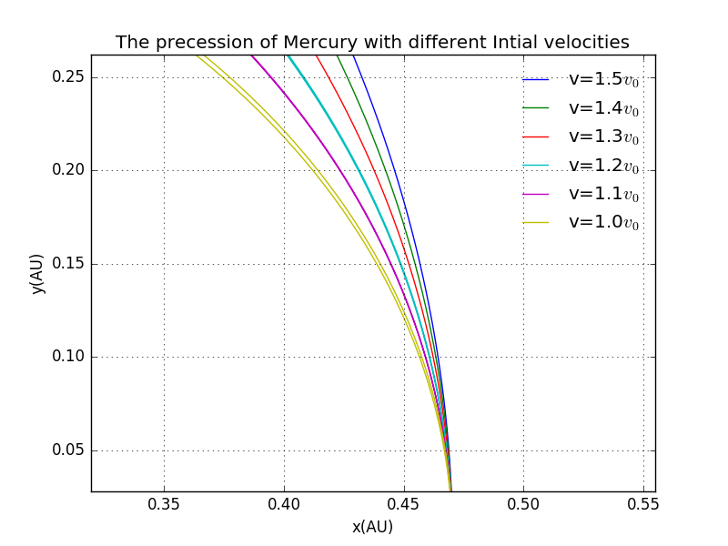
It is clearer to plot them in just one plot.

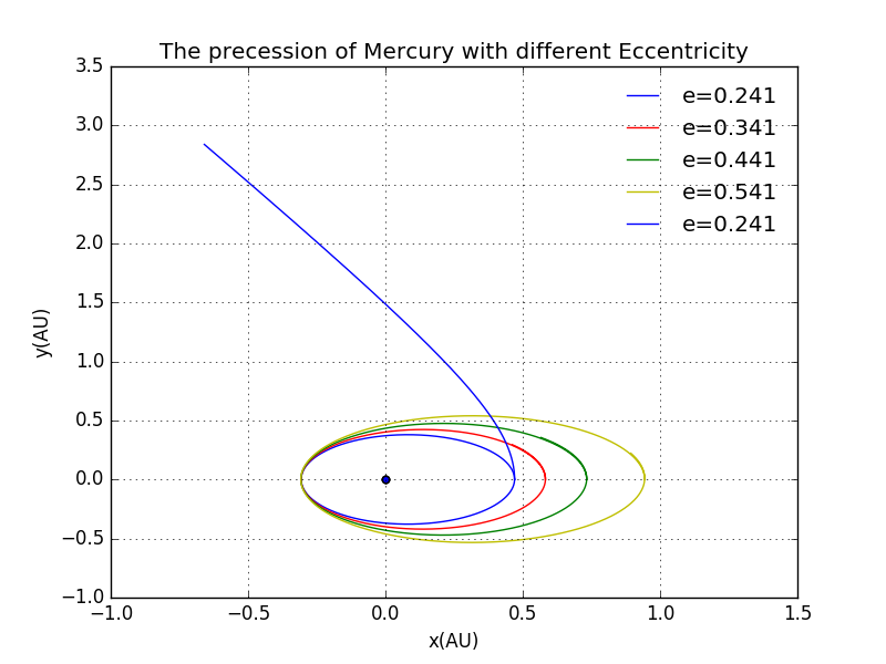
As illustrated before,the intial velocity $v_0$ required for a closed orbital movement is precisely required for $v_0=\sqrt{\frac{GM_S (1-e)}{a(1+e)}}$.The misbehave of the blue line in following plot suggests a intial velocity $v=2v_0$.As displayed,it will be ejected from the solar system with sufficint time.

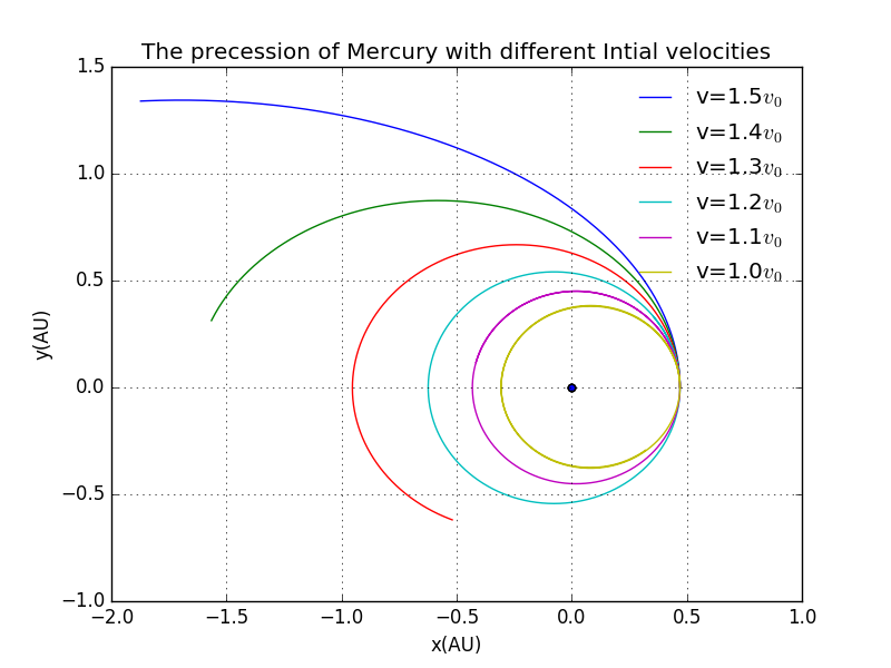
Here we set different intial velocity $v_0$ to investigate the behavior of Mercury.As the increment of $v_0$ the Mercury will at last went away from the solar system with the second universal velocity.

Details

5.2 Characteristic of various $\beta$

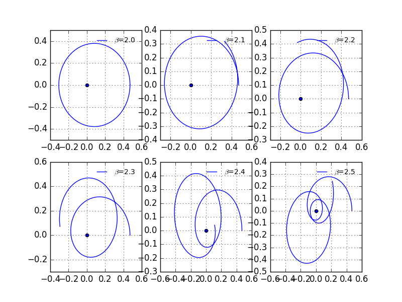
Illustrated before,we expect the law to be inverse-square law.But what if we change the $\beta$ not equal to 2 ?The following plot gives varous values of $\beta$.We shall see,except the situation where $\beta=2.0$,the trajectory is not closed.

With longer period it becomes:

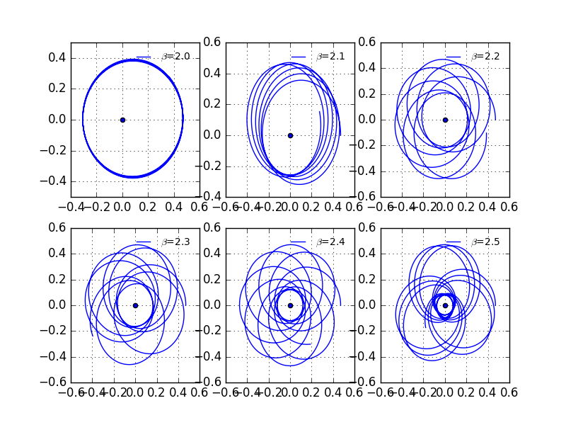
A more precise situation where $\beta=2.1$.Obviously,the path is not closed.

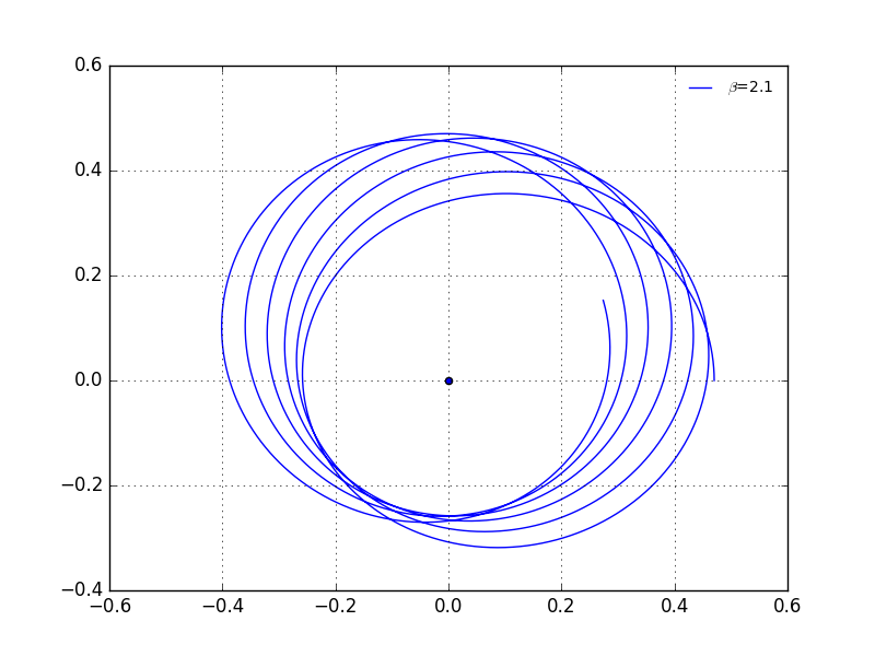
Different time duration of $\beta=2.5$

5.3 The precession calculation.

Here we plot the plot of $\theta$ versus time with $\alpha=0.0008$

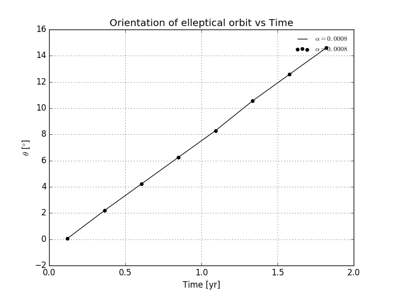
Having changed the value of $\alpha$ we observe some misbehave of the curves.

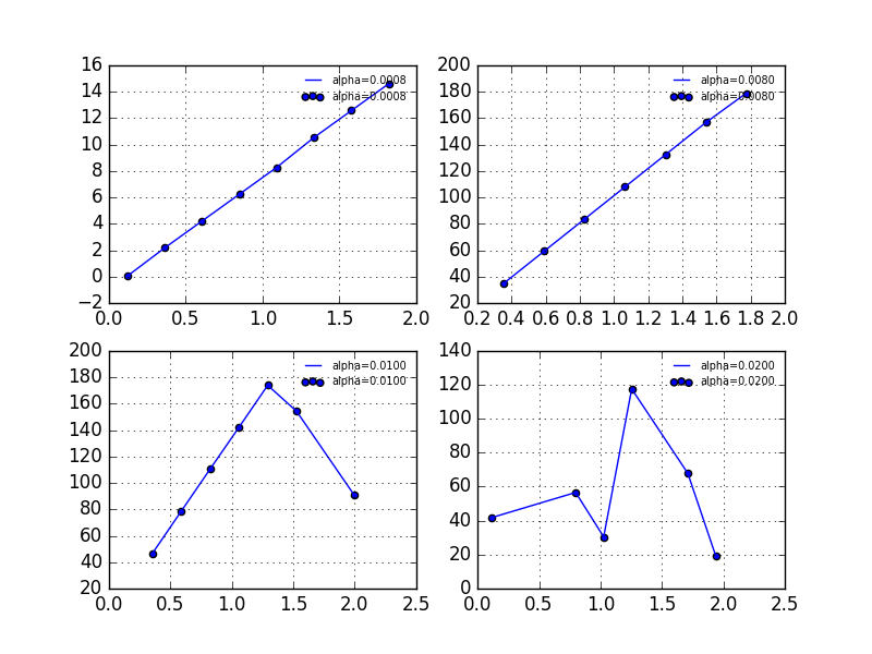
Let us return to the precession of the perihelion of Mercury.We shall see the slope of the lines remains constant as predicted.

6 Vpython Part

6.1 Souce code

Adapted fromVpython Contributed Program

from visual import *
#from Numeric import *
print '''
Simple solar system model showing the orbits of the planets
Note: In this version the orbits are not tilted so
      the longitude of the ascending node is not correct.
created by Lensyl Urbano, Jan. 2006.
'''
class orbit:
    def __init__(self,e=0.0,rad=1.0, mu=10.0, planet_size=1.0, period=365,
                 inclination=0.0, lap=0.0, frate=10000000):
        self.orbit_path = curve(color=color.green,radius=0.075)
        self.planet = sphere(color=color.yellow,radius=planet_size)
        if e >= 1.0:
            e = 0.99
        if e < 0.0:
            e = 0.0
        fx = 2.0 - 2.0*min(abs((1-e*e)/(1-e)), abs(-(1-e*e)/(1+e)))
        self.fx = fx
        self.e = e
        self.rad = rad
        self.dangle = 360./period
        self.inclination = inclination
        self.lap = lap
        for i in range(int(period)+1):
            rate(frate)
            theta = radians(float(360.*i/period))
            #h_sq = a*(1-e*e)*mu
            r = (1-e*e)/(1-e*cos(theta))
            nx = rad*(r*cos(theta) - fx)
            ny = rad*r*sin(theta) 
            #print i, f, r, cos(theta), sin(theta), nx, ny
            #nz = rotate(vector(nx,ny,0.0), angle=inclination, 
            posi = rotate(vector(nx,ny,0.0), angle=radians(inclination), axis=(0,1,0))
            posi = rotate(posi, angle=radians(lap), axis=(0,0,1))
            self.orbit_path.append(pos=posi)
            self.planet.pos=posi
        self.angle = 0.0
    def re_draw(self,e=0.0,rad=1.0,mu=10.0, frate=10000000):
        #redraw last path
        if e >= 1.0:
            e = 0.99
        if e < 0.0:
            e = 0.0
        fx = 2.0 - 2.0*min(abs((1-e*e)/(1-e)), abs(-(1-e*e)/(1+e)))
        self.fx = fx
        self.e = e
        self.rad = rad
        for i in range(361):
            rate(frate)
            theta = radians(float(i))
            #h_sq = a*(1-e*e)*mu
            r = (1-e*e)/(1-e*cos(theta))
            nx = rad*(r*cos(theta) - fx)
            ny = rad*r*sin(theta) 
            self.orbit_path.pos[i]=vector(nx, ny, 0.0)
    def move_planet(self):
        self.angle = self.angle + self.dangle
        #to show the planet orbiting the Sun
        theta = radians(float(self.angle))
        r = (1-self.e*self.e)/(1-self.e*cos(theta))
        nx = self.rad*(r*cos(theta) - self.fx)
        ny = self.rad*r*sin(theta) 
        posi=rotate(vector(nx,ny,0.0), angle=radians(self.inclination), axis=(0,1,0))
        posi = rotate(posi, angle=radians(self.lap), axis=(0,0,1))
        self.planet.pos = posi
#class proton:
origx = 0
origy = 0
w = 704 #+4+4
h = 576 #+24+4
scene.width=w
scene.height=h
scene.x = origx
scene.y = origy
mu = 10.0 #gravitational acceleration
#e = 0.6 #eccentricity
#a = 10.0 #distance of sun from center of elipse
# to draw an elipse
nucleus = frame()
p1 = sphere(color=color.white, frame=nucleus)
#orbitor = sphere()
e1 = orbit(e=0.50, rad=15.0, mu=mu, 
              planet_size=0.5, period=365,
              lap=90)
##e2 = orbit(e=0.0, rad=15.0, mu=mu, 
##              planet_size=1.0, period=365,
##              lap=0, inclination=90)
runtime = 0.0
framerate = 60
pick = None
while 1:
    rate(framerate)
    runtime += 1.0/framerate
    e1.move_planet()
##    e2.move_planet()

6.2 Results with single elleptical orbit

6.3 The Solar System(Parts of solar system)

7 Acknowledgement

1.Wikipideia.The free encyclopedia
2.SHIXING WANG.
3.ZONG YUE