张梓桐计算物理期末论文

RANDOM WALK RELATED ANALYSIS

张梓桐 2014301020005 弘毅班
PDF版本更加清晰：1.百度网盘；2.GITHUB

1 Abstract

In the previous section,we have gone through too many deterministic system.Here we are going to discsus the random process,which means,random walk.We gave a brief introduction to the process of random walk in 1D,2D and 3D.Additionally,we summarize the diffusion model.At last,the DLA cluster model is presented.
[Key word]: Random Walk; Simulation; Diffusion; Cluster

2 Background

For most of the time,our focus has been put on the issue with deterministic system,such as the projectile motion of the cannon ball,or the electric potential.Nevertheless,why don't we shift our thinking and consider something that is not so absolute,say,random.

3 Random Walk

As far as I am concerned,apart from the uncertanity principle in the Quantum Mechanics,everything ''underlying'' physics of the system may be deterministic,our incomplete knowledge may force us to resort to a stastical,i.e.,stohastic desctiption.For example,we could list a large number of differential equations which we could in principle solve.But out computer is limited in its computational ability and what we really require is a satistical description instead of any details of every particle at any given time.Now the random system comes to its significance when we deal with system with very large number of ''degree of freedom''.$^{[1]}$

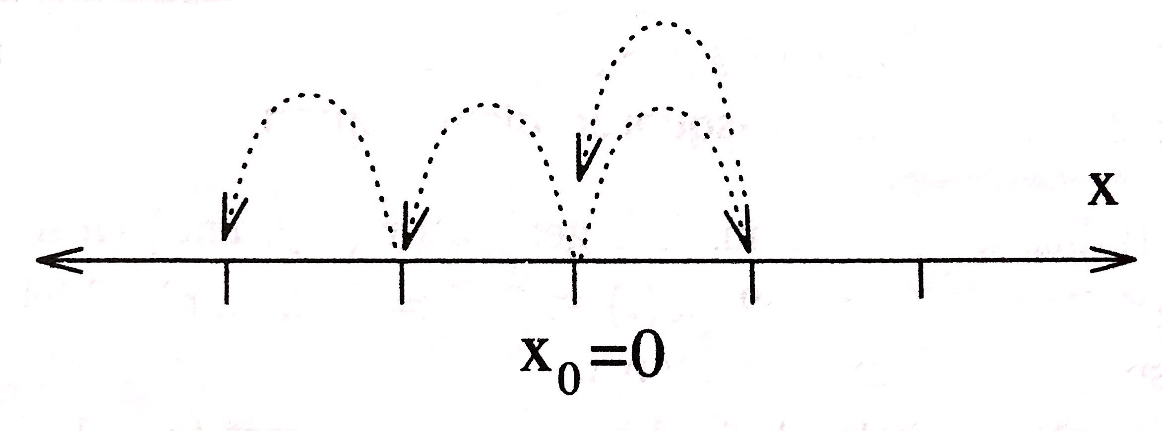
Here ,we formally introduce the concept of random walk.A random walk is a mathematical object which describes a path that consists of a succession of random steps.$^{[2]}$ .The simplist situation involves a walker that is able to take steps of length unity along a line.

Lattic Random Walk

A popular random walk model is that of a random walk on a regular lattice, where at each step the location jumps to another site according to some probability distribution. In a simple random walk.$^{[7]}$
Here in our discussion,we pick the walking direction to be $(\pm1,0)$ and $(0,\pm1)$ with given probablity.As the stimulation,that is to say,the step number increase,this simple situation can easily be applied to random walk in any direction.

3.1 Random Walk Analysis For 1D

3.1.1 The Walking With Fixed Step Length

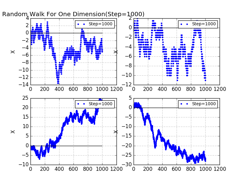
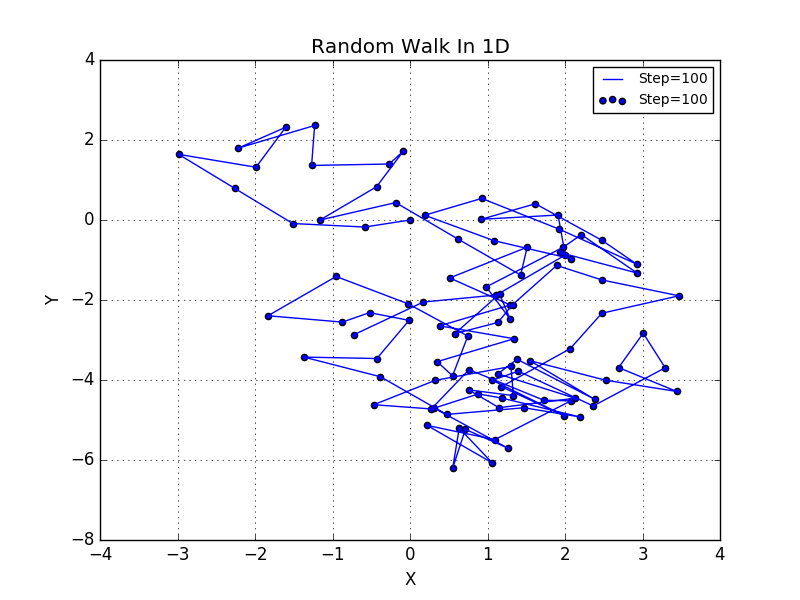
Firstly,we stimulate the random walk for one dimension,1D for abbrevation.We take the step to be 1000 steps without the lossing of generality.In the figure,we see no obvious regular pattern in each results.And that is the exactly what we have expected before.

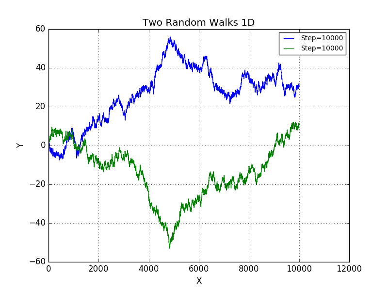
In order to illustrate more explicitly,we take the step to be 10000 steps.It is obvious that no distinct pattern is shown here.

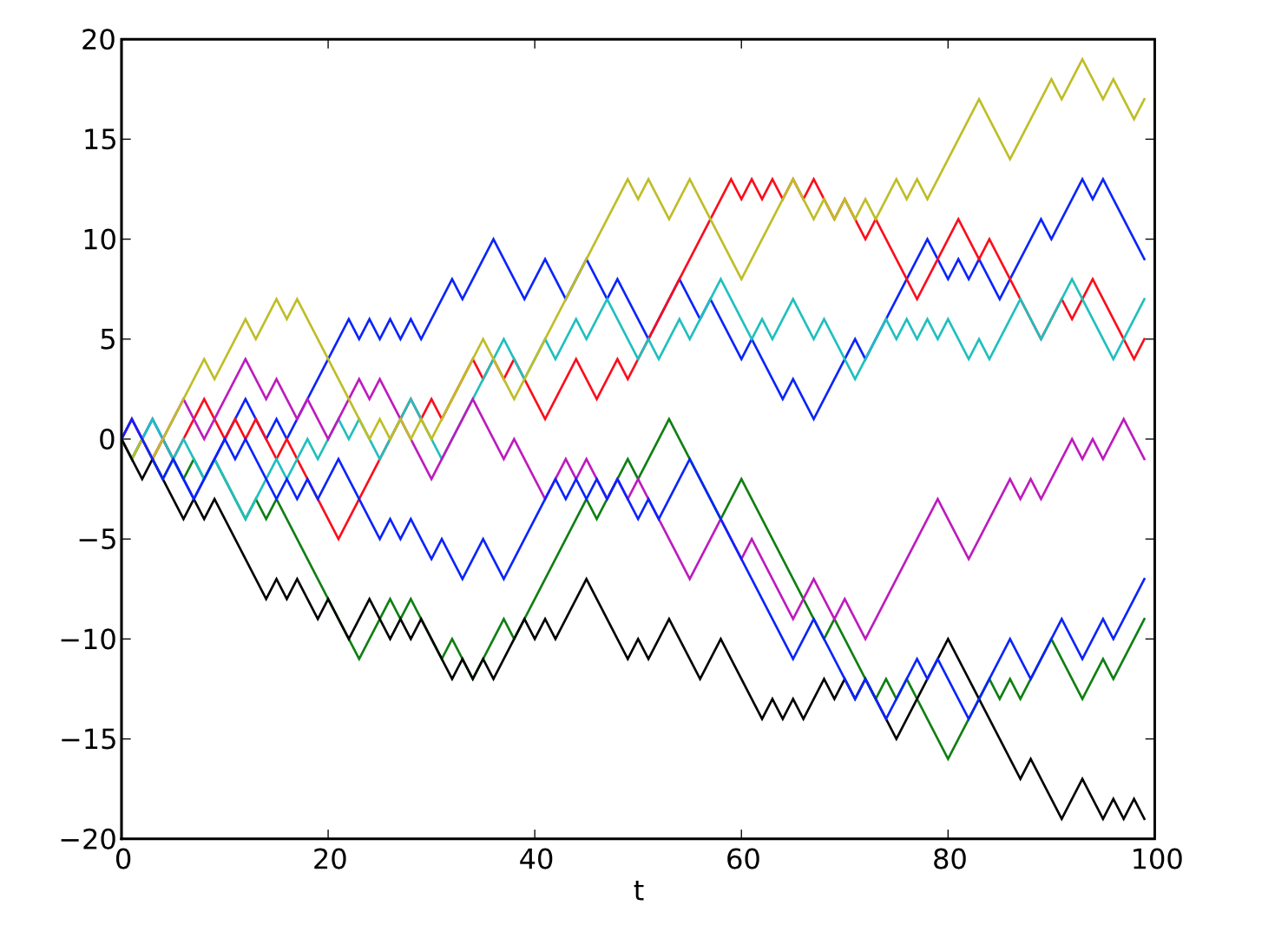
Eight times stimulation of a 1D random walk.

This walk can be illustrated as follows. A marker is placed at zero on the number line and a fair coin is flipped. If it lands on heads, the marker is moved one unit to the right. If it lands on tails, the marker is moved one unit to the left. After five flips, the marker could now be on 1, −1, 3, −3, 5, or −5. With five flips, three heads and two tails, in any order, will land on 1. There are 10 ways of landing on 1 (by flipping three heads and two tails), 10 ways of landing on −1 (by flipping three tails and two heads), 5 ways of landing on 3 (by flipping four heads and one tail), 5 ways of landing on −3 (by flipping four tails and one head), 1 way of landing on 5 (by flipping five heads), and 1 way of landing on −5 (by flipping five tails). See the figure below for an illustration of the possible outcomes of 5 flips.$^{[3]}$

3.1.2 The $<x_n^2>$ Plot With Fixed Step Length

As we might have expected,due to the equality of the probablity of the drunnk walker turning right or turning left,the average walk might cancel each other after being averaged,which leads to:

$$\begin{eqnarray*} <x_n>=0 \end{eqnarray*}$$
However,a more interesting and informative quantity is $<x_n^2>$,the average of the square of the displacement after n steps.Some results shall be presented later.But here we are going to show you a formula that has been teseified by thousands of time in the 1D random walk model.
$$\begin{eqnarray*} <x_n^2>=2Dt \end{eqnarray*}$$
where t is the time,which here is just equal to the step number;the factor $D$ is known as the diffusion constant.\footnote{The factor 2 is inserted here so that the continuum limit of this random walk will reduce to the standard diffusion equation.}

For such a particle we know that $x=vt$,so its distance from the origin grows linearly with time.Thus we obtain $\sqrt{<x^2>}\propto t^\frac{1}{2}$.Actually,the results for D can be obtained analytically.

$$\begin{eqnarray*} x_n=\sum_{i=1}^{n}s_i \end{eqnarray*}$$
where $s_i$ is the displacement of the $i$th step.
$$\begin{eqnarray*} x_n^2=\sum_{i=1}^{n}(\sum_{j=1}^{n}s_js_i) \end{eqnarray*}$$
Since the steps are independent of each other,the terms $s_i s_j$ with $i\neq j$ will be $\pm 1$ with equal probaility.Thus we find:
$$\begin{eqnarray*} <x_n^2>=\sum_{i=1}^{n}s_i^2=n \end{eqnarray*}$$

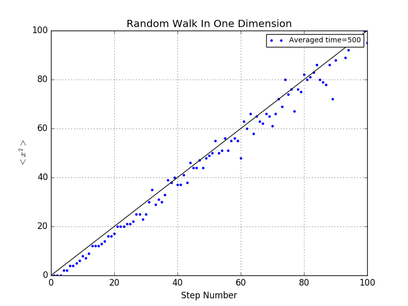
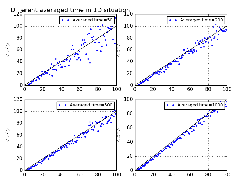
If we choose different stimulation times for each step number,say ,from $50$ to $1000$.It is evident that the scattered dots is approximating the fit line of $y=x$.This phenomenon is universially acknowledged as the statistical error.Given the chance that we make infinite walks every for every step,those scattering points is just the straigh line.

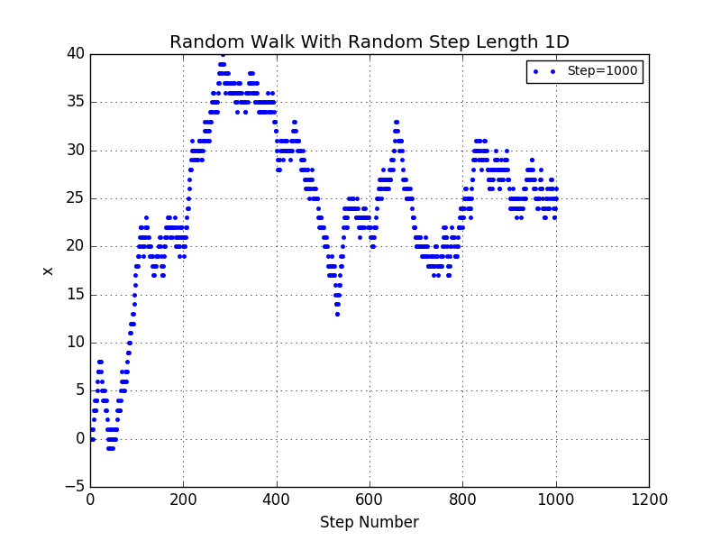
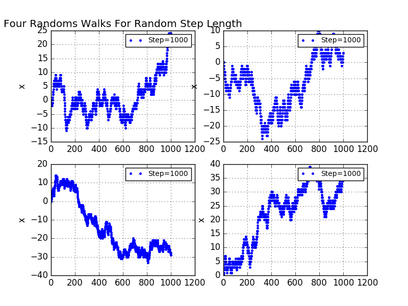
3.1.3 The Walking With Random Step Length

Up to this point we have considered the most simple random-walk model.There are many ways to generalize the model to make it more realistic.One way is to allow the steps to be of random length.Here are some results:

We also find the diffusive behavior,which accords well with the fixed step random walk

Here we plot two separate random walks for random length.

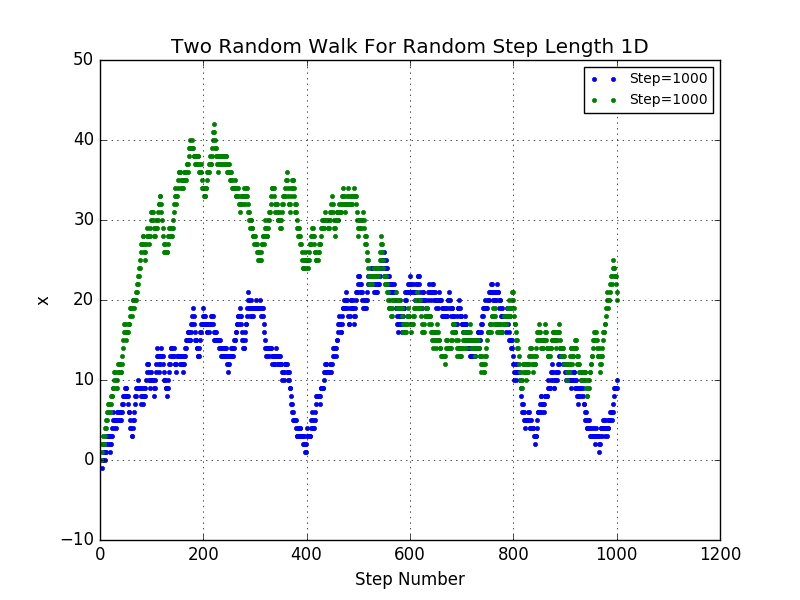
Four random walks for random length

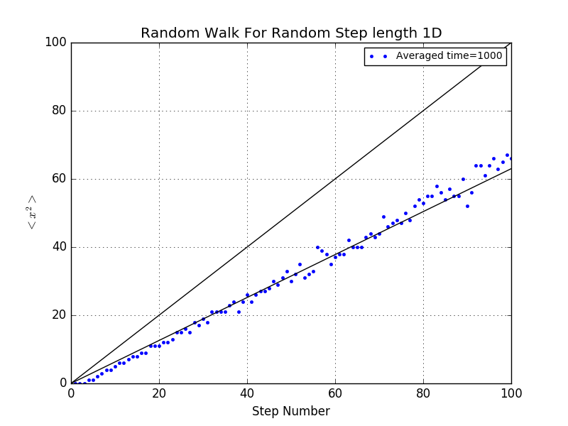
3.1.4 The $<x_n^2>$ Plot With Random Step Length

However,the $<x_n^2>$ is being changed as the changing of step length,we observe that the slope of the fit line,that is,from $y=x$ shifting to $y=\frac{1}{2}x$.Worth mentioning,the value of $D$ can also be calculated analytically.But right here,we are not going to illustrate it explicitly.

3.2 Random Walk Analysis For 2D

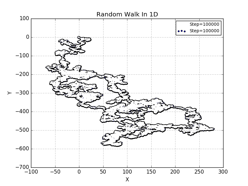
Simliar to the situation we have discussed in 3.1,now the drunker can walk in a two-dimensional world,though not relaistic enough,but closer to the realistic situation:

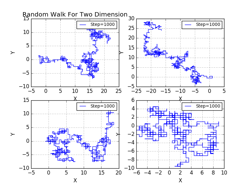
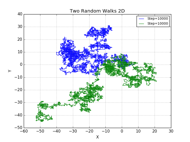
We are unable to observe any pattern just like in 1D situation with two random walks.

3.3 Random Walk Analysis For 3D

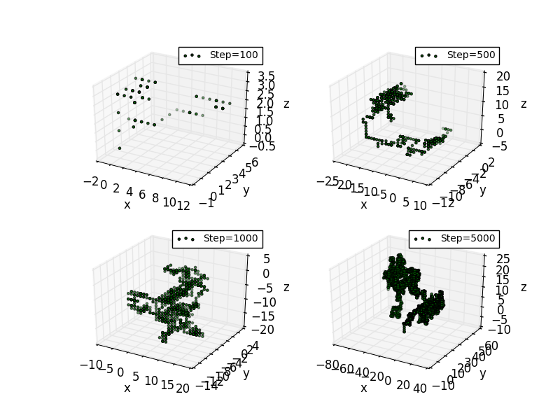
Another obvious generalization is to allow the walker to move in three dimensions.
There is an intersesting of whether the drunk man able to go back to where he begin?This is the 2-dimensional equivalent of the level crossing problem discussed above. It turns out that the person almost surely will in a 2-dimensional random walk, but for 3 dimensions or higher, the probability of returning to the origin decreases as the number of dimensions increases.$^{[4]}$
The resuts is shown below.

In higher dimensions, the set of randomly walked points has interesting geometric properties. In fact, one gets a discrete fractal, that is, a set which exhibits stochastic self-similarity on large scales.

3.4 Further Analysis Regarding $<x_n^2>$

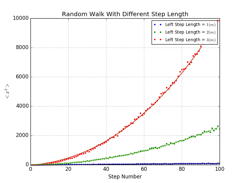
Up to now,we have considering the situation in which the step of going right and left are equal,and the step length is equal to unity.As the situation described above is of extremely symmetry.What if we destroy the symmetry,for example:

We take the probability of turning left less than that of turning right.You can imagine this situation happens if the drunker hurts one of his legs! Now with the disappearance of symmetry,we observe a parabola,which indicate the drunker is more likely to go faster away from the origin than the equal probability situation.

Similiarly,we assume the drunker had a longer left legs,and he was able to go further and faster away from the origin than the equal leg one does.

4 Diffusion

The reason why we are going to discuss about the process of diffusion is obvious,that is,the diffusion are equvailent to diffusion.Now we are going to discuss the diffusion in details.

Diffusion is the net movement of molecules or atoms from a region of high concentration (or high chemical potential) to a region of low concentration (or low chemical potential).

Considering the case in which you put a cream in your coffee.You will definitely find that the cream spread slowly until it loose all of its shape and merge totally.
What we really care about is the density of particle $\rho(x,y,z,t)$,which can be conveniently defined if the system contains a large number of particles.The density is then propotional to the probability per unit time $t$.Now we give the equation that both $P$ and $\rho$ satsifies.

$$\begin{eqnarray*} P(i,j,k)=\frac{1}{6}[P(i+1,j,k,n-1)+P(i-1,j,k,n-1)+P(i,j+1,k,n-1)+P(i,j-1,k,n-1)+P(i,j,k+1,n-1)+[P(i,j,k-1,n-1)] \end{eqnarray*}$$
The equation is what we usually called as diffusion equation in the form of finite difference.This suggests taking the continuum limit,which leads to:
$$\begin{eqnarray*} \frac{\partial P(x,y,z,t)}{\partial t}=D\nabla ^2P(x,y,z,t) \end{eqnarray*}$$
Now we substitute the probability $P$ with the density $\rho$,and rearrange the equation to express the density at time step $n+1$ in terms of $\rho$ at step $n$ we find:
$$\begin{eqnarray*} \rho(i,n+1)=\rho(i,n)+\frac{D\Delta t}{(\Delta x)^2}[\rho(i+1,n)+\rho(i-1,n)-2\rho(i,n)] \end{eqnarray*}$$

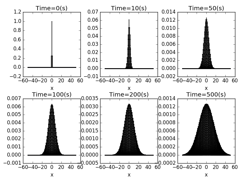
Now we are going to show you the schematic solutions of the diffusion equation at several different times.The Gaussian distribution broadens with time,but the area under the curve,which is equal to the total number of particles,does not change

$$\begin{eqnarray*} \rho(x,t)=\frac{1}{\sigma}exp[-\frac{x^2}{2\sigma ^2}] \end{eqnarray*}$$

4.1 The Diffusion In One Dimension

Here we plot the time evolution calculated from the the diffusion equation in one dimensions at $t=0$ to $t=500(s)$Note that the vertical scales are different in the different plots;the maxium value of the density decreased as t increased,which keep the total number of particles fixed.

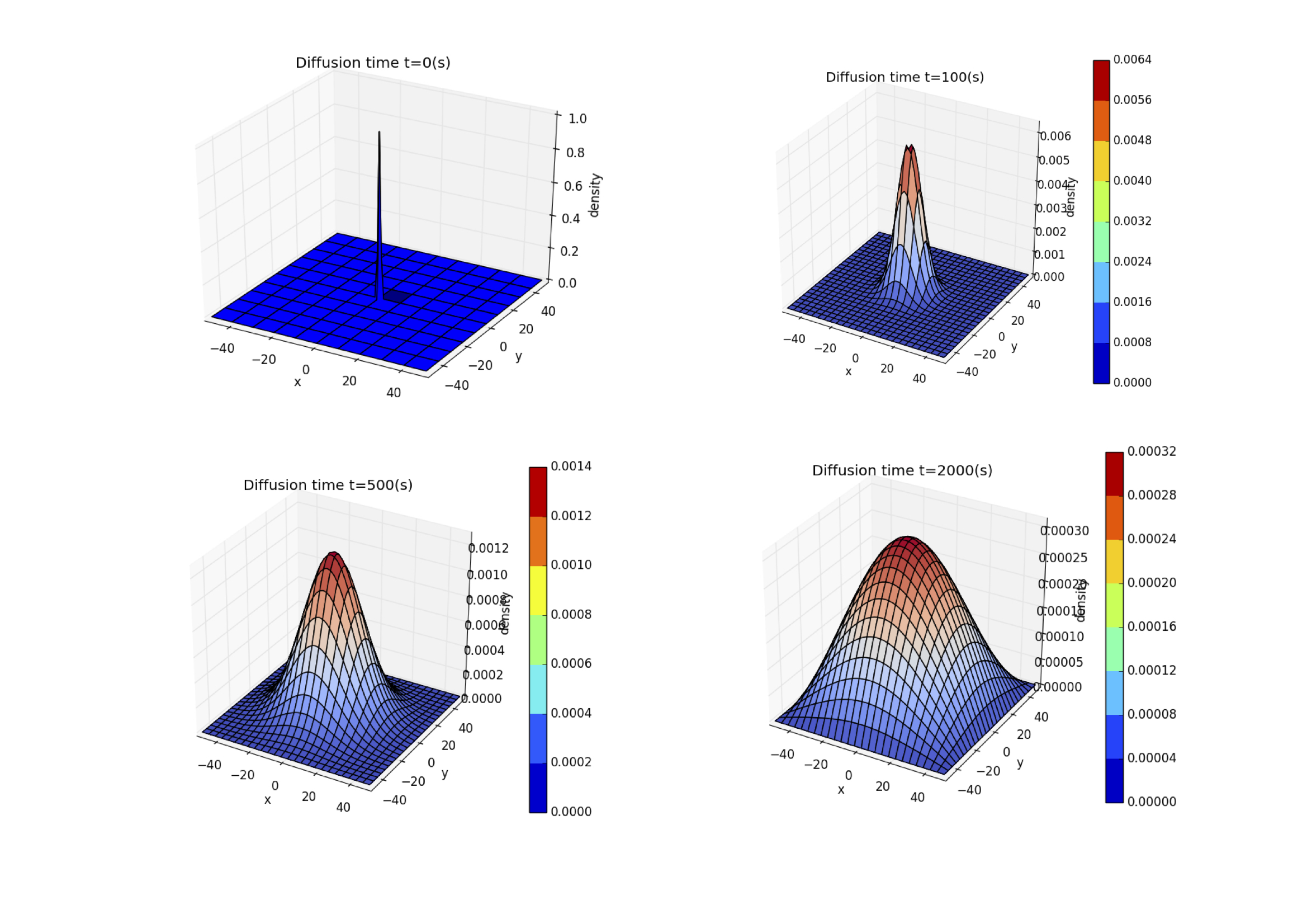
4.2 The Dirac Diffusion In Two Dimension

To visualize the diffusion process,we take a 3D plot to indicate the 2D diffusing process.Here we choose the Dirac function as intial condition.It is obvious that the vertical scale is diminishing as the one dimension situation.After a really long time ,say,$2000(s)$(I have to say this process really takes longer time than I have expected!) the solution almost reach equilibrium,for the density distribution is rather flat.(The highest point only contributes 0.00032)

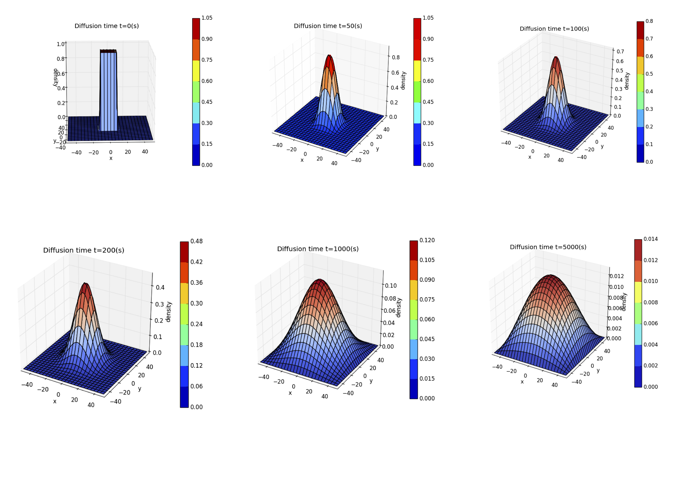
4.3 The Square-Cream Diffusion In Two Dimension

Time evolution calculated from the diffusion equation in two dimensions.At $t=0$,all of the particles were confined to clump at the center of the system.The distribution at $t=50$,$t=100$,$t=200$,$t=1000$ and $t=5000$ are shown.The region shown here covers the range $|x,y|\leq 50$.

5 Cluster Growth Models

Another interesting random process,which turns out to be closely related to random walks,concerns the growth of cluster,such as snow flakes and soot particle.There existing two main kinds of cluster growth model.One is the Eden cluster growth model,and the other is Diffusion-Limited aggregation,or DLA.

5.1 Eden Cluster

The Eden growth model describes the growth of specific types of clusters such as bacterial colonies and deposition of materials. These clusters grow by random accumulation of material on their boundary. These are also an example of a surface fractal.$^{[5]}$The way the Eden Cluster is formed is illustrated as follow:

We begin by placing a seed particle at the origin;this is our initial cluster.The we choose one of these perimeter sites at random and place a particle at the chosen location.The cluster now contains two particles and a correspondingly larger perimeter.

5.2 DLA Cluster$^{[6]}$

Diffusion-limited aggregation (DLA) is the process whereby particles undergoing a random walk due to Brownian motion cluster together to form aggregates of such particles.

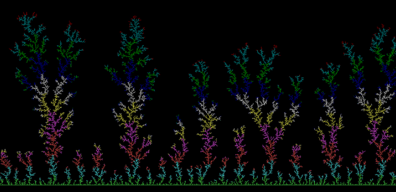
The growth rules for DLA clusters are as follows.We again start with a seed particle at the origin.We then release a particle at a randomly chosen location that is some distance away from the seed and let it performs a random walk.If this walker lands on a perimeter site,it sticks there and becomes part of the cluster.

Here is a DLA obtained by allowing random walkers to adhere to a straight line. Different colors indicate different arrival time of the random walkers.

5.2.1 DLA Simulation

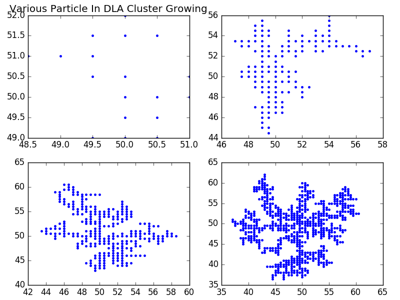
The filled circles are sites in the cluster.Here we have generated 1000 particles.It is likely that there might be some localized source of the small particle.This is perfectly reasonable models and could be interesting depending in part on possible connections to real system.

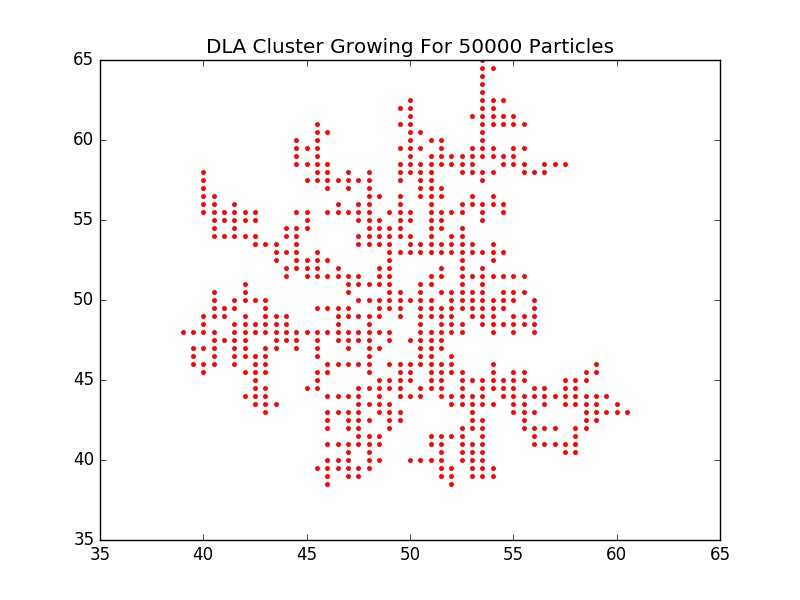
Now we generate 50000 particles.We can observe better understanding of the DLA Cluster Growth model

To observe the difference of generating particles number.

5.2.2 DLA Dimensionality

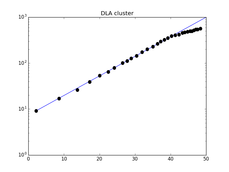
Let us consider how we might measure the dimensionality of an object.Apart from the previous definition,it is instructive to construct an operational definition for dimensionality.

$$\begin{eqnarray*} m(r)\propto r^{d_f} \end{eqnarray*}$$
where $d_f$ is the effectice of fractal dimensionality of the object.Since taking the logarithm of both sides of the above equation we obtain:
$$\begin{eqnarray*} \log m\propto d_f \log r \end{eqnarray*}$$

However,the curves flatton out for large $r$.This is due to the finite size of the clusters.For very large measuring circles,the entire cluster will be inside the circle,and in this case $m(r)$ will be independent of $r$.The dimensionality of DLA Cluster is $d_f \approx 1.65$.

6 Conclusion

6.1 Random Walk

• We are unable to clone two identical random walk pattern,which means this process is absolutely random.
• The average of $<x_n>$ is zero,however,$<x_n^2>$ might be propotional to step number.
• If the probability or the step length or turning right or left are not symmetric,ther may appear to be a parabola.

6.2 Diffusion

• The Gaussian distribution broadens with time,but the area under the curve,which is equal to the total number of particles,does not change.
• For a give initial condition,the details may not be deterministic,however,the overall pattern is determined by the law of diffusion.

6.3 DLA Cluster Growth

• DLA Cluster Growth Model describes well with the realistic situation.
• We are not able to clone any one of the results.
• The dimensionality of DLA Cluster is $d_f \approx 1.65$.

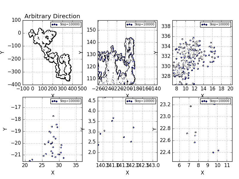
7 Other Interesting Situation

Here we try something new in the Random Walk section.We do not assume the direction to be neither $(±1,0)$ nor $(0,±1)$,instead,we take the direction to be arbitrary so that this match with the realistic situation much better.

8 Source Code

Please check:
1.Random Walks Calculation.py
2.Diffusion.py
3.DLA cluster.py

9 Reference

$[1]$ Nicholas J.Giordano;Hisao Nakanishi,Computational Physics,second edition,Pearson Education.2007-12
$[2]$ From Wikipedia, the free encyclopedia,Random Walk.
$[3]$ From Wikipedia, the free encyclopedia,One Dimension Random Walk.
$[4]$ Pólya's Random Walk Constants, Mathworld.wolfram.com. Retrieved 2016-11-02.
$[5]$ Barabasi, Albert-Laszlo; Stanley, Harry Eugene (1995). Fractal Concepts in Surface Growth. Cambridge University Press. pp. 123–125. ISBN 0-521-48318-2.
$[6]$ Tiger Zhou for his conduction in cluster growth model.
$[7]$ Pal, Révész (1990) Random walk in random and non random environments, World Scientific