张梓桐计算物理第九次作业

1 Problem

3.30

2 Abstract

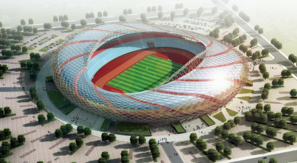
As the previous dicusssion of two kinds of situation in the chaos,we will consider one more chaotice model in this paper.Here we consider the problem of a ball moving without friction on a horizontal table.Apart from that,we are also going to consider the so-called Stadium shape,which can be described as in books.We will dicsuss the phase plot,the trajectory plot ant the divergence plot with the stadium ball.

3 Background

3.1 The moving part

Except for the collisions with the walls,the motion fo the billiard is quite simple.Between collisions the velocity is constant so we have:

$$\begin{eqnarray*} \frac{dx}{dt}=v_x \quad \frac{dy}{dt}=v_y \end{eqnarray*}$$
where $v_x$ and $v_y$ change only through collisions with the walls.These equation can be solved using our usual Euler alogrithm.

3.2 The collision part

As for the collision part,we have a solution.
After each step we must check to see if there has been a collision with one of the walls,that is,if the newly calculated position puts the billiard off the table.When this happens the program must backtrack to locate the position where the collision occurred.There are several ways to do this.One way is to back the billiar up to the position at the previous time step and then use a much smaller time step,so as to move the billiard in much smaller steps.When the billiard then goes off the table again,we take the location after that iteration to be the point of collision.

$$\begin{eqnarray*} \vec v_{i,\perp}=(\vec v_i\cdot \widehat n)\widehat n \end{eqnarray*}$$
$$\begin{eqnarray*} \vec v_{i,\parallel}=\vec v_i-\vec v_{i,\perp} \end{eqnarray*}$$
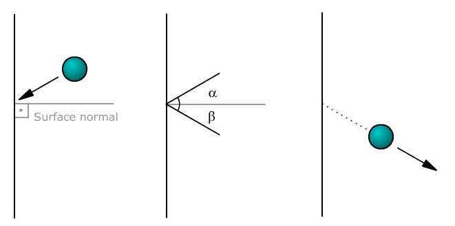
After we have the components of $\vec v_i$ we can relect the billiard:
$$\begin{eqnarray*} \vec v_{f,\perp}=-\vec v_{i,\perp} \end{eqnarray*}$$
$$\begin{eqnarray*} \vec v_{f,\parallel}=\vec v_{i,\parallel} \end{eqnarray*}$$
Here are photos that indicate those equations explicitly.

What if there are many balls? When shall learn next chapter.

3.3 Chaos Theory

Chaos theory is the field of study in mathematics that studies the behavior of dynamical systems that are highly sensitive to initial conditions—a response popularly referred to as the butterfly effect. Small differences in initial conditions (such as those due to rounding errors in numerical computation) yield widely diverging outcomes for such dynamical systems, rendering long-term prediction impossible in general. This happens even though these systems are deterministic, meaning that their future behavior is fully determined by their initial conditions, with no random elements involved. In other words, the deterministic nature of these systems does not make them predictable. This behavior is known as deterministic chaos, or simply chaos. The theory was summarized by Edward Lorenz as:

Chaos: When the present determines the future, but the approximate present does not approximately determine the future.

Logistic Tops Mixing:

Six iterations of a set of states passed through the logistic map. (a) the blue plot (legend 1) shows the first iterate (initial condition), which essentially forms a circle. Animation shows the first to the sixth iteration of the circular initial conditions. It can be seen that mixing occurs as we progress in iterations. The sixth iteration shows that the points are almost completely scattered in the phase space. Had we progressed further in iterations, the mixing would have been homogeneous and irreversible. The logistic map has equation . To expand the state-space of the logistic map into two dimensions, a second state, , was created as , if and otherwise.

3.4 Lorentz Attractor

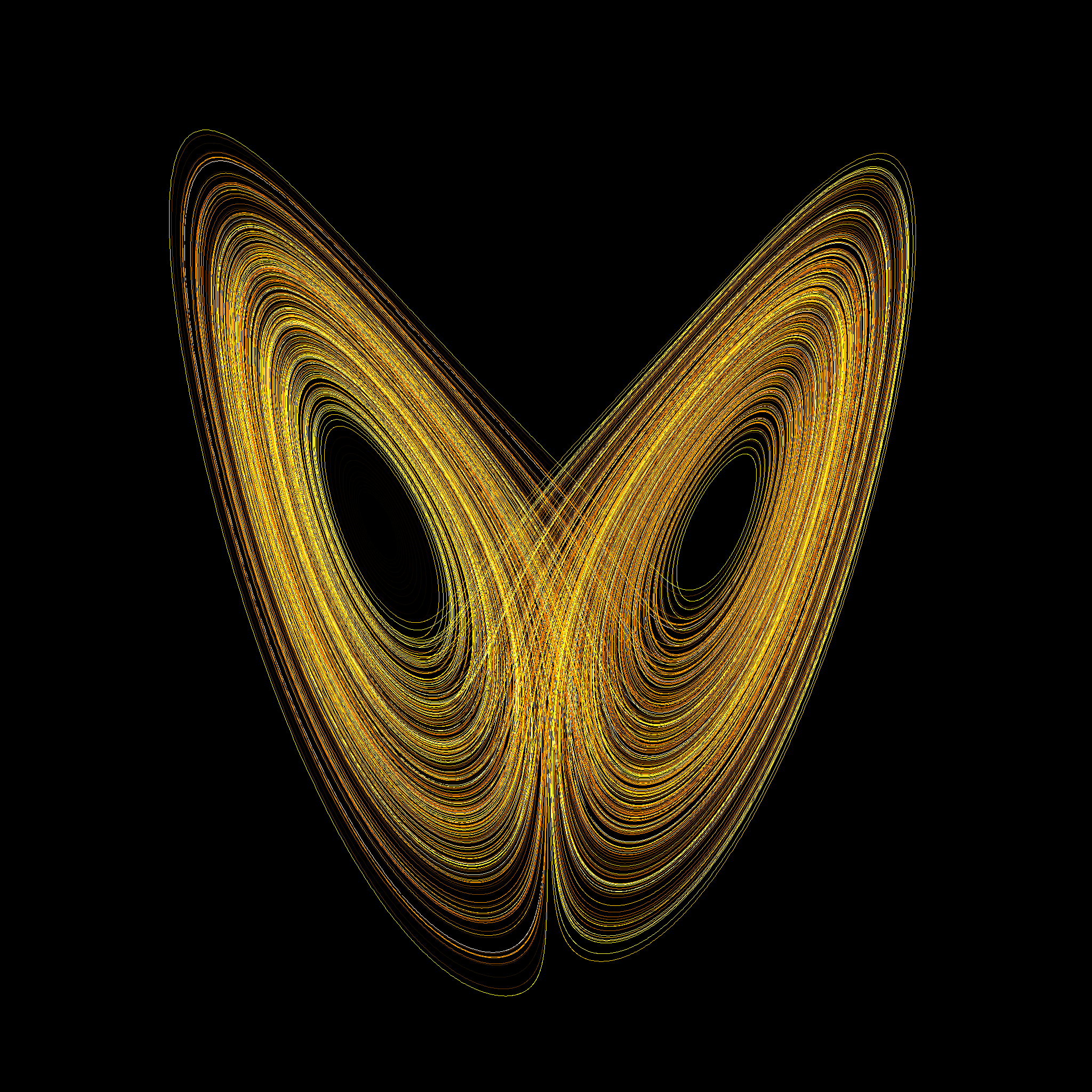
Having been aware of them,we can safely say that it will not be hard for us to draw all the plot we needed.One points need to be mentioed.A hall mark of a chaotic system is an extreme sensitivity to intial conditions.This property is also found in the Lorentz attractor:

It look just like a butterfly.The Lorenz system is a system of ordinary differential equations (the Lorenz equations, note it is not Lorentz) first studied by Edward Lorenz. It is notable for having chaotic solutions for certain parameter values and initial conditions. In particular, the Lorenz attractor is a set of chaotic solutions of the Lorenz system which, when plotted, resemble a butterfly or figure eight.

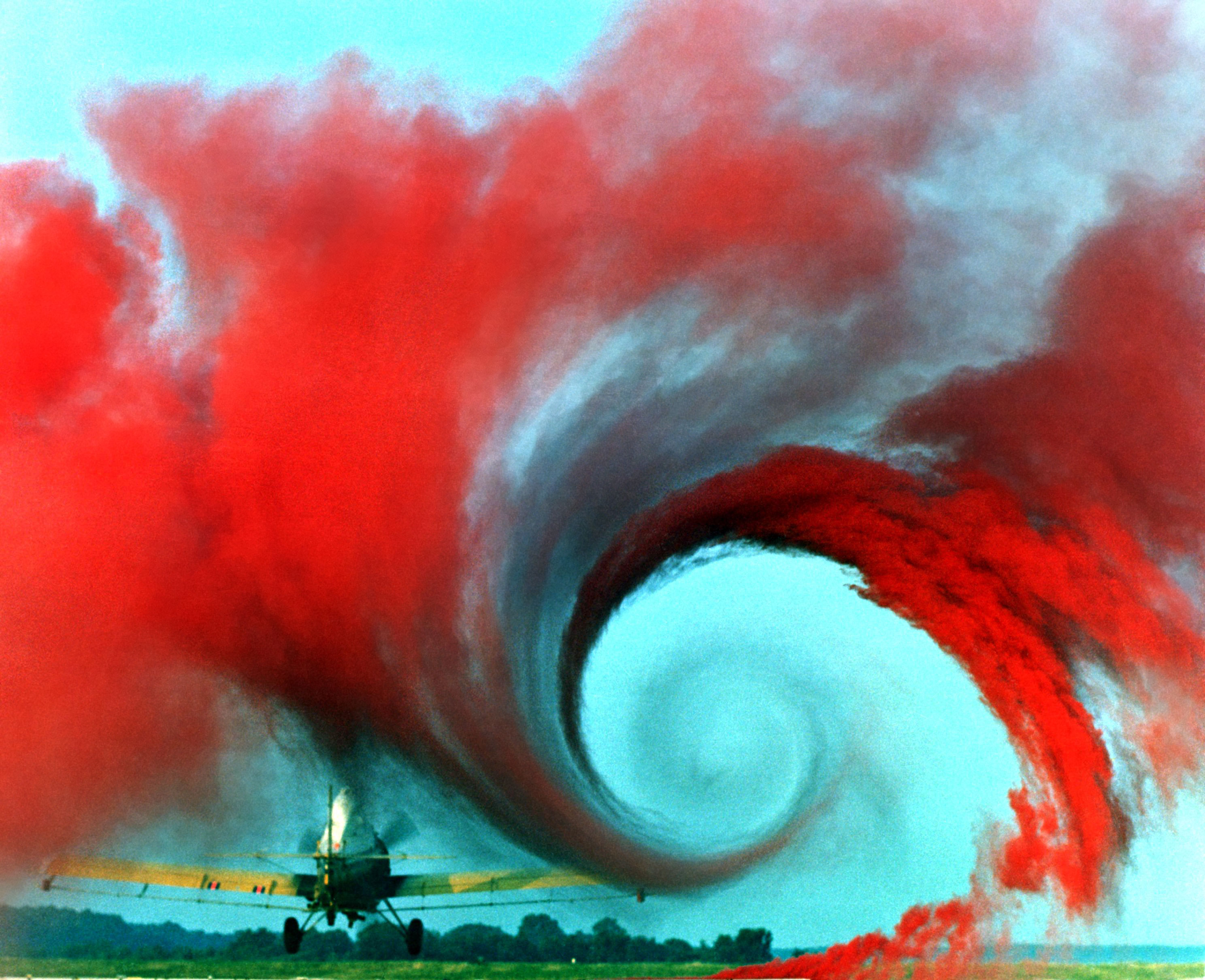
Here is a photo of actual turrbulance!You may not want this.It is an airplane vortex.

4 Main body

Source Code 1 for stadium
Source Code 2 for Lyapunov exponent

5 Results

5.1 Perfect Circle

5.1.1 Trajectory plots

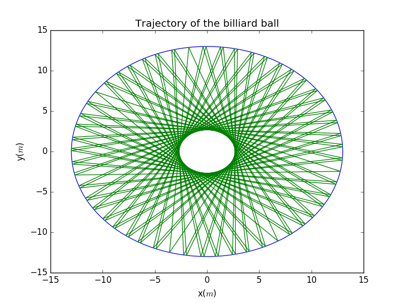
Before rendering the stadium ball,we first check the situation in the perfect sphere.As you can see,it's perfect after hundreds of collisions.Additionally,there are some ponits in the plot can never be reached no matter how many collisions occurred.

With the previous notation of the backwarf trace.Here we would like to investigate the precesion of the time step that may make a influence on the accuracy of the plot.Here we use the precesion $\frac{1}{10}$, $\frac{1}{100}$, $\frac{1}{1000}$, $\frac{1}{10000}$ the previous time step.But we see no obvious differnece after the precesion reaches$\frac{1}{1000}$ and later.

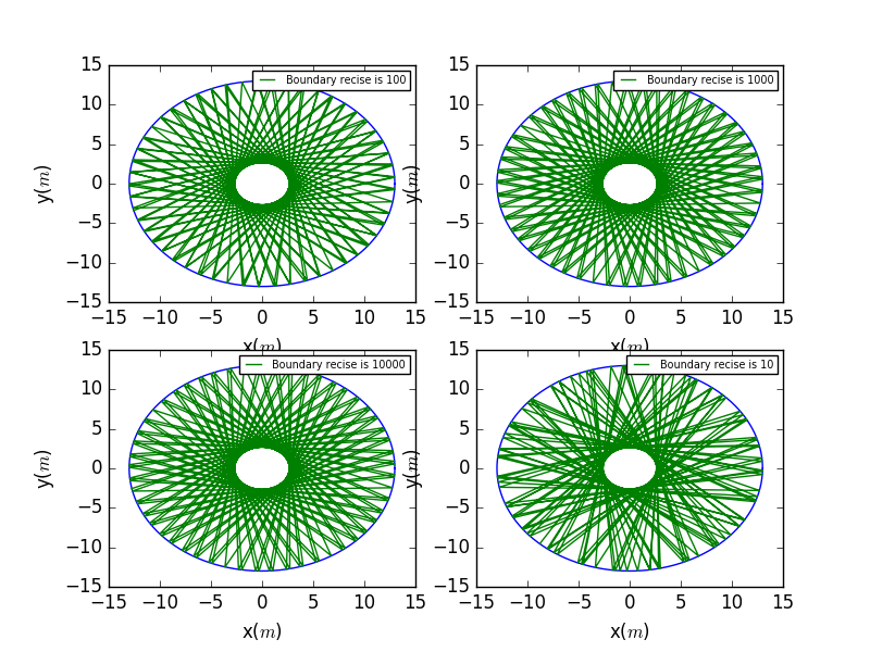
Here we use the precesion $\frac{1}{50}$, $\frac{1}{100}$, $\frac{1}{150}$, $\frac{1}{200}$ the previous time step.Now we can see evidently the progessively accurate plots.

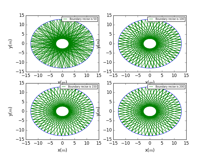
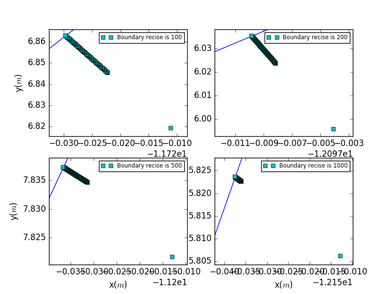
How about we check the details of the collide points for further observation.It is eviednt that the higher the precesion,the closer the reflection points near the boundary.

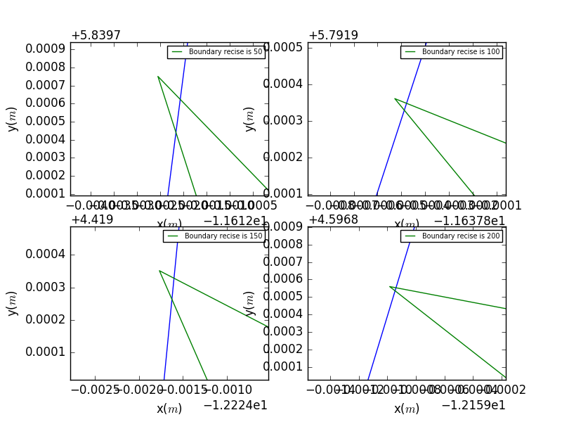
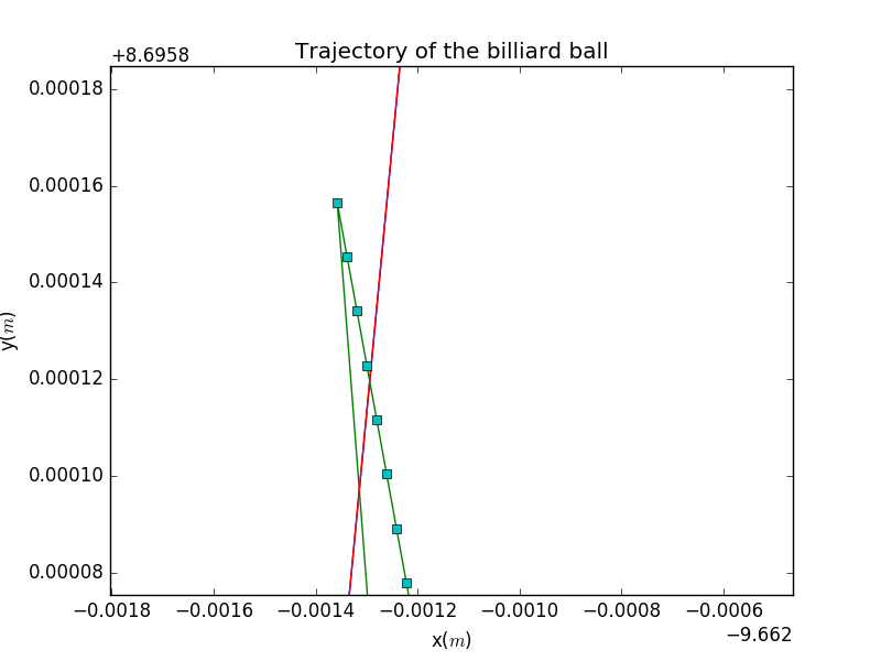
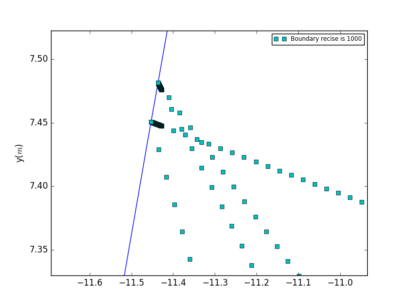
In this plots,we specify a particular plots.With the difference in density of points,we know the bcakward program is actually working well!

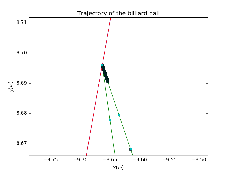
From this plot,we acquire a better understanding of the actually process of the collision.The collision points are not actually lies in the boundary,but span a distance that is too small too be found.In that sense,we regared this process as reflection.

5.1.2 Phase Plots

The phase plots:

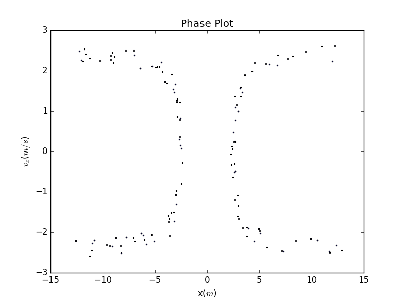
For further description,we draw the phase plot.That is $v_x-x$ plots.We see the points gradually becomes more with the increment of collision times.

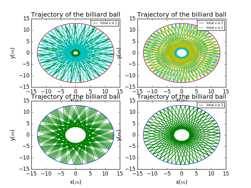
5.1.3 Stange things 0.0

Interestingly,here are some plots with different intial position of x,you may see in the plots, the area that can not be reached is changing(the radius of blank area) via the changing of intial position.

5.2 Stadium Ball

5.2.1 Trajectory Plots

To see an exgarrate $\alpha$= 0.5.It look just like a stadium


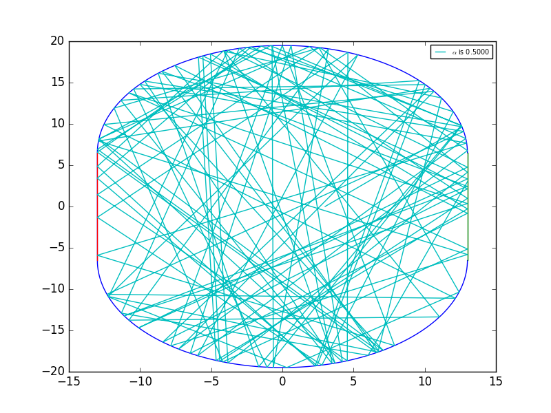
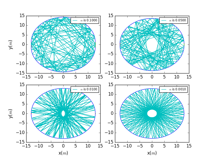
Having discussed the perfect balls,let us look at the stadium ball.Here we change the $\alpha$ to $0.1$, $0.05$, $0.01$, $0.001$. It's obviously that the higher the $\alpha$,the more chaotic the trajectory is,which means the area that may never be reached before shall be reached now.But as the $\alpha$ is becoming smaller,it behaves like the perfect circle boundary.With the limit $\alpha \rightarrow 0$,it will finally becomes a circle boundary.

Worth mentioning,the more precise the backward program,the more chaotic the trajectory may be.Here we use the precesion $\frac{1}{100}$, $\frac{1}{200}$, $\frac{1}{500}$, $\frac{1}{1000}$ the previous time step.

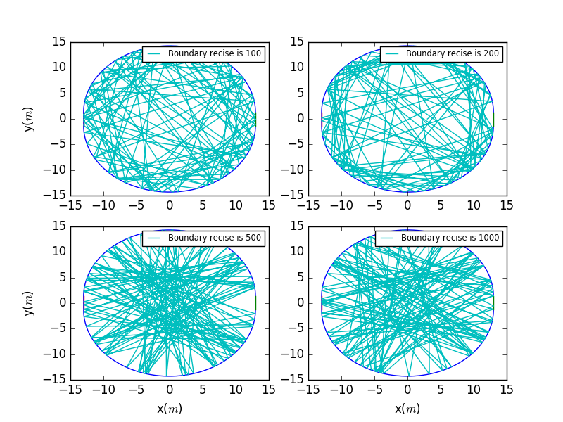
The conclusion also hold that the higher the precesion,the closer the reflection points near the boundary.

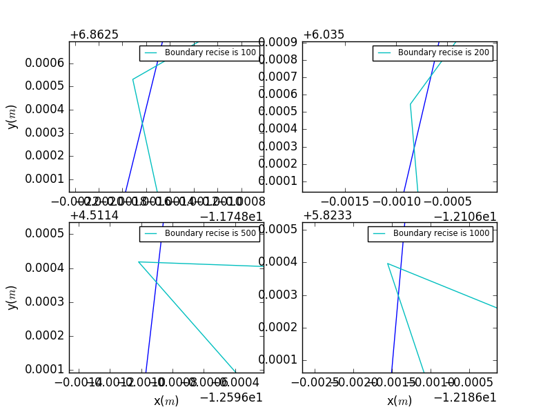
Some details of the refelction points:

A comparision of different precesion.It is clear that as the precesion becomes higher,the closer the dense points near the boundry.

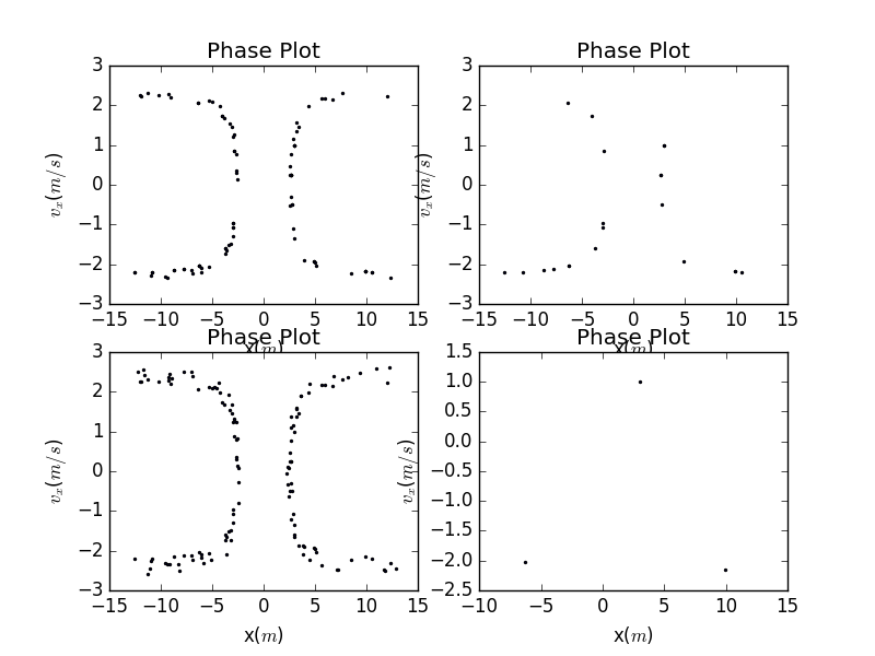
5.2.2 Phase Plots

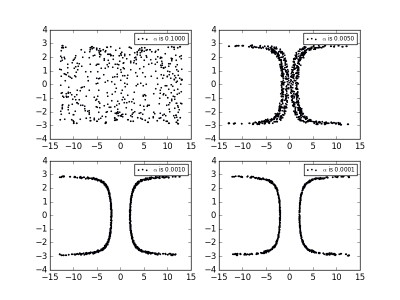
Now it's time to make the phase plots.We choose $\alpha$ to be $0.1$, $0.05$, $0.01$, $0.001$ in order to see the variation of the plots.We can see with the increase of the value of $\alpha$,the plots is becoming more alike the perfect circular one.But with low value of $\alpha$, it seems that all the points may be reached throughout the space.

5.2.3 Lyapunov exponent

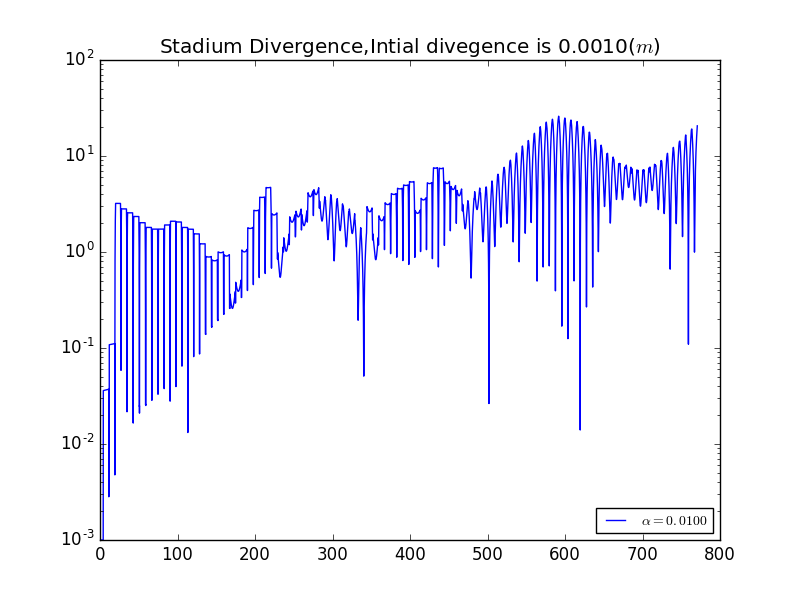
Now we consider the Lorentz attractod effect of two nearly seperated balls.We plot the distance between two billiards as a function of time.The billiards were on a chaotic table ($\alpha$=0.01) and were given the same intial velocities,but were seperated with a small distance.Here are plots with differnet seperation of $0.05m$, $0.01m$, $0.005m$.Here you can see the varies a lot when the time is big enough.

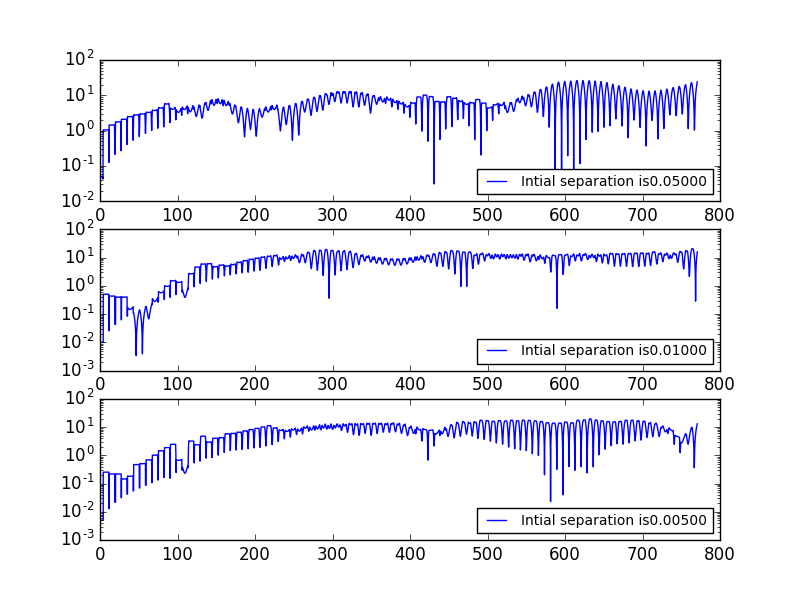
The billiards seperation shows a very sharp dip after about every unit of time.These dips occur when the billiards collide with the walls,as this causes their trajectories to cross.The overall seperation is seen to increase very rapidly with time.

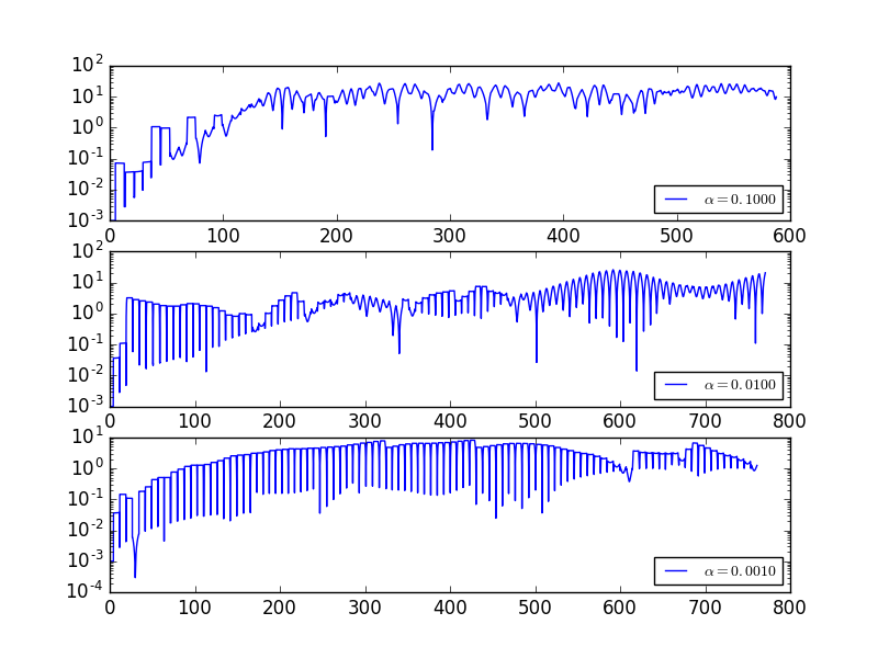
Plots wit differnet $\alpha$.We set $\alpha$ to be $0.1$, $0.01$, $0.001$.

6 VPython display

from visual import *
side = 4.0
thk = 0.3
s2 = 2*side - thk
s3 = 2*side + thk
wallR = box (pos=( side, 0, 0), size=(thk, s2, s3),  color = color.green)
wallL = box (pos=(-side, 0, 0), size=(thk, s2, s3),  color = color.green)
wallB = box (pos=(0, -side, 0), size=(s3, thk, s3),  color = color.green)
wallT = box (pos=(0,  side, 0), size=(s3, thk, s3),  color = color.green)
wallG = box (pos=(0,0,-2*side),size=(s3,s3,s3),color=color.green)
ball = sphere(pos=(0.2,0,0), color=color.white, radius = 0.5, make_trail=True, retain=200)
ball.trail_object.radius = 0.07
ball.v = vector(0.5,0.3,0.4)
side = side - thk*0.5 - ball.radius
dt = 0.5
t=0.0
while True:
  rate(100)
  t = t + dt
  ball.pos = ball.pos + ball.v*dt
  if not (side > ball.x > -side):
    ball.v.x = -ball.v.x
  if not (side > ball.y > -side):
    ball.v.y = -ball.v.y
  if not (side>ball.z>-side):
      ball.v.z=-ball.v.z

We obtain the plot in 2-Dimension.

Also, there is 3-Dimension.!30

7 Acknowledgement

1.Thanks to Wikipedia.
2.Thanks to Yu Kang,since we discuss the details of the program.
3.Zong Yue for his VPython program.