计算物理第十次作业Problem4.8

---

摘要

上次作业研究了桌球的碰撞问题，而此次作业将重点放在了大家熟悉又陌生的太阳系中。

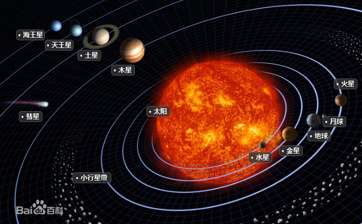
背景

已知在天体运动中天体遵循万有引力定律：

$$F_G=\frac{GM_SM_E}{r^\beta}$$
将太阳运动分解为x，y轴方向可以得到： $$\frac{dv_x}{dt}=-\frac{GM_Sx}{r^3}$$ $$\frac{dx}{dt}=v_x$$ $$\frac{dv_y}{dt}=-\frac{GM_Sy}{r^3}$$ $$\frac{dy}{dt}=v_y$$
由Euler-Cromer方法可以处理上面式子，并取初始条件为x=a(1+e),y=0,$V_y=V_{min}$同时有：

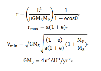
此时一个简单的模型已经出来了，但不足之处有未考虑相对论等效应。

正文

1. 行星椭圆运动

程序为：

import pylab as pl
import math
class Solar_system :
    def __init__(self,i=0,initial_x=1,initial_y=0,initial_vx=0,initial_vy=2*math.pi,\
                 total_time=10, time_step=0.002, radius=1):
        self.x=[initial_x]
        self.y=[initial_y]
        self.vx=[initial_vx]
        self.vy=[initial_vy]
        self.r=[radius]
        self.time=total_time
        self.dt=time_step
        self.t=[0]
    def run(self):
        _time=0
        while(_time<self.time):
            self.vx.append(self.vx[-1]-4*pow(math.pi,2)*self.x[-1]/pow(self.r[-1],3)*self.dt)
            self.x.append(self.x[-1]+self.vx[-1]*self.dt)
            self.vy.append(self.vy[-1]-4*pow(math.pi,2)*self.y[-1]/pow(self.r[-1],3)*self.dt)
            self.y.append(self.y[-1]+self.vy[-1]*self.dt)
            self.t.append(_time)            
            _time += self.dt
    def show_results(self):
        pl.plot(self.x,self.y)
        pl.title('Solar system')
        pl.xlabel('x(AU)')
        pl.ylabel('y(AU)')
        pl.legend()
        pl.show()
a = Solar_system()
a.run()
a.show_results()  

运行结果为：

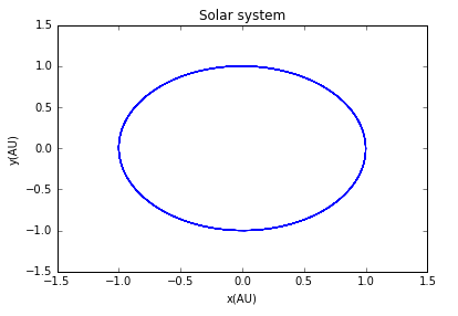
当改变e值时即可改变轨道形状，可得结果：

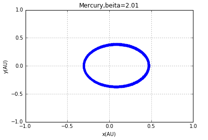
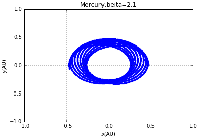
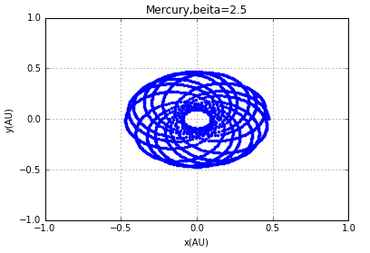
2 不同β运动轨迹

以水星为例，取β=2、2.01、2.1、2.5的轨道轨迹，程序如下：

import pylab as pl
import math
def initial(a,e,MP,beta):
    MS=2*10**(30)
    x0=a*(1+e)
    y0=0
    vx0=0
    vy0=2*math.pi*math.sqrt((1-e)/(a*(1+e))*(1+MP/MS))
    return [x0,y0,vx0,vy0,beta]
class orbits():
    def __init__(self,x0,y0,vx0,vy0,beta):
        self.x=[x0]
        self.y=[y0]
        self.vx=[vx0]
        self.vy=[vy0]
        self.dt=0.001
        self.t=[0]
        self.steps=2000
        self.r=[]
        self.beta=beta
    def calculate(self):
        for i in range(self.steps):
            self.r.append(math.sqrt(self.x[i]**2+self.y[i]**2))
            temp_vx=self.vx[i]-4*math.pi**2*self.x[i]*self.r[i]**(-self.beta-1)*self.dt
            self.vx.append(temp_vx)
            temp_x=self.x[i]+self.vx[i+1]*self.dt
            temp_vy=self.vy[i]-4*math.pi**2*self.y[i]*self.r[i]**(-self.beta-1)*self.dt
            self.vy.append(temp_vy)
            temp_y=self.y[i]+self.vy[i+1]*self.dt
            self.x.append(temp_x)
            self.y.append(temp_y)
            self.t.append(self.t[i]+self.dt)
        return self.x,self.y
    def show_result(self):
        pl.plot(self.x,self.y,".")
        pl.xlabel('x(AU)')
        pl.ylabel('y(AU)')
        pl.xlim(-1,1)
        pl.ylim(-1,1)
        pl.title("Mercury,beita=2")
        pl.grid(True)
        pl.show()
I=initial(0.39,0.206,2.4*10**(23),2)
a=orbits(I[0],I[1],I[2],I[3],I[4])
a.calculate()
a.show_result() 

运行结果为：

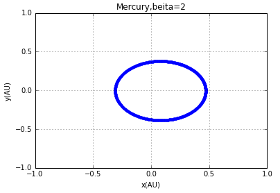
改变β值即有：

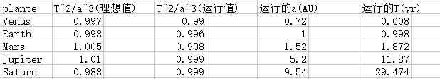
3 验证开普勒第三定律与理想值的比较

程序为：

import pylab as pl
import math
def initial(a,e,MP):
    MS=2*10**(30)
    x0=a*(1+e)
    y0=0
    vx0=0
    vy0=2*math.pi*math.sqrt((1-e)/(a*(1+e))*(1+MP/MS))
    return [x0,y0,vx0,vy0]
class orbits():
    def __init__(self,x0,y0,vx0,vy0):
        self.x=[x0]
        self.y=[y0]
        self.vx=[vx0]
        self.vy=[vy0]
        self.dt=0.001
        self.t=[0]
        self.steps=300001
        self.r=[]
        self.x2=[]
        self.y2=[]
        self.t2=[]
    def calculate(self):
        for i in range(self.steps):
            self.r.append(math.sqrt(self.x[i]**2+self.y[i]**2))
            temp_vx=self.vx[i]-4*math.pi**2*self.x[i]*self.r[i]**(-3)*self.dt
            self.vx.append(temp_vx)
            temp_x=self.x[i]+self.vx[i+1]*self.dt
            temp_vy=self.vy[i]-4*math.pi**2*self.y[i]*self.r[i]**(-3)*self.dt
            self.vy.append(temp_vy)
            temp_y=self.y[i]+self.vy[i+1]*self.dt
            self.x.append(temp_x)
            self.y.append(temp_y)
            self.t.append(self.t[i]+self.dt)
            if self.y[i+1]<0:
                self.y2.append(self.y[i+1])
                self.x2.append(self.x[i+1])
                self.t2.append(self.t[i+1])
        a=(self.x[0]-self.x2[0])/2
        T=self.t2[0]*2
        print(a,T,T**2/a**3)
        return self.x,self.y,self.x2,self.y2
    def show_result(self):
        pl.plot(self.x,self.y,".")
        pl.xlabel('x(AU)')
        pl.ylabel('y(AU)')
        pl.xlim(-1.5,1.5)
        pl.ylim(-1.5,1.5)
        pl.title('simulation of elliptical orbit')
        pl.show()
I_v=initial(0.72,0.007,4.9*10**(24))
v=orbits(I_v[0],I_v[1],I_v[2],I_v[3])
v.calculate()
v.show_result()
I_e=initial(1,0.017,6*10**(24))
e=orbits(I_e[0],I_e[1],I_e[2],I_e[3])
e.calculate()
e.show_result()
I_ma=initial(1.52,0.093,6.6*10**(23))
ma=orbits(I_ma[0],I_ma[1],I_ma[2],I_ma[3])
ma.calculate()
ma.show_result()
I_j=initial(5.2,0.048,1.9*10**(27))
j=orbits(I_j[0],I_j[1],I_j[2],I_j[3])
j.calculate()
j.show_result()
I_s=initial(9.54,0.056,5.7*10**(26))
s=orbits(I_s[0],I_s[1],I_s[2],I_s[3])
s.calculate()
s.show_result()

运行结果为：

结论

由上面运行结果可以看出基本可以模拟出行星运动的轨迹，同时也可以开普勒第三定律验证时与理想值还是有一定差距的，而误差来源可能是每一步的时间距离以及点数选取太少。

致谢

感谢陆文龙同学的耐心帮助。