张梓桐计算物理第十二次作业

1 Problem

5.1& 5.4& 5.5

2 Abstract

The partial differential equation is of physicists' great interest for its widely applicaiton in decribing physical systems. Jacobi method and simultaneous over relaxation method are two algrithm that keep a balance of the simplicity for comprehension and accuracy of computation. Here in this passage,we are going to discuss the relation and difference with differnet methods in tackling same problem.

3 Background

3.1 Electrical Field

An electric field is a vector field that associates to each point in space the Coulomb force that would be experienced per unit of electric charge, by an infinitesimal test charge at that point.1 Electric fields converge and diverge at electric charges and can be induced by time-varying magnetic fields. The electric field combines with the magnetic field to form the electromagnetic field.--Wikipedia,the free Encylopeida.

3.2 Jacobi Method

In numerical linear algebra, the Jacobi method (or Jacobi iterative method) is an algorithm for determining the solutions of a diagonally dominant system of linear equations. Each diagonal element is solved for, and an approximate value is plugged in. The process is then iterated until it converges.

Particularly,in our dicussion in this passage,Jacobi Method can be easily expressed as below:

$$\begin{eqnarray*} V_{new}(i,j)=\frac{1}{4}[V_{old}(i+1,j)+V_{old}(i-1,j)+V_{old}(i,j+1)+V_{old}(i,j-1)] \end{eqnarray*}$$

3.3 Gauss-Sideal Method

In numerical linear algebra, the Gauss–Seidel method, also known as the Liebmann method or the method of successive displacement, is an iterative method used to solve a linear system of equations. It is named after the German mathematicians Carl Friedrich Gauss and Philipp Ludwig von Seidel, and is similar to the Jacobi method.

Particularly,in our dicussion in this passage,Gauss-Seidel Method can be easily expressed as below:

$$\begin{eqnarray*} V_{new}(i,j)=\frac{1}{4}[V_{old}(i+1,j)+V_{new}(i-1,j)+V_{old}(i,j+1)+V_{new}(i,j-1)] \end{eqnarray*}$$

Worth mentioning,whilw the performance if the Gauss-Seidel akgorithm is better than that of the Jacobi method,the imporvement is only modest.It turns out that the number of iterations required for convergence with the Gauss-Siedel method is smaller,but only by a factor of 2.

But the benefits in Gauss-Seidel method is obvious,cause there is no need for us to save the old values seperately.In other words, the updating can be performed in place with $V(i,j)$ using an algorithm of the form.

$$\begin{eqnarray*} V(i,j)=\frac{1}{4}[V(i+1,j)+V(i-1,j)+V(i,j+1)+V(i,j-1)] \end{eqnarray*}$$

3.4 Simulatneous over-relaxation(SOR)

With this method ,the problem of relatively low convergence rate can be easily solved.Let $V^*(i,j)$ be the new value of calculated.Then the change of $V$ is represented as:

$$\begin{eqnarray*} \Delta V(i,j)=V^*(i,j)-V_{old}(i,j) \end{eqnarray*}$$
However,we have seen in our previous examples that this choice of $\Delta V(i,j)$ is too conservative.So to speed up convergence we will change the potential by a larger amount calculated according to:
$$\begin{eqnarray*} V_{new}(i,j)=\alpha \Delta V^*(i,j)+V_{old}(i,j) \end{eqnarray*}$$
where $\alpha$ is a factor that measures how much we "over-relax".Choosing $\alpha=1$ tuekds the Gauss-Seidel method.It turns out that if $\alpha\geq 2$ , the method does bit converge.The best choice of $\alpha$ is
$$\begin{eqnarray*} \alpha \approx \frac{2}{1+\pi/L} \end{eqnarray*}$$

4 Source Code

1.Electric field
2.Potential

There are some points in my code that I want to illustrate:

v=np.zeros((100,100))

The sentence above is to set a $100\times100$ grids for the upcoming potential value,and we intialize them to be zero all.

self.q=np.zeros((100,100))
self.q[49:50,49:50]=1

Those sentences above are to set the unit charge at position (50,50),and the other part of the space to be zero.

v[40:60,60]=1
v[40:60,40]=-1

Those sentences above are to set the intial condition of $V=+-1$ in both $y=60(grid)$ and $y=40(grid)$ with length extended from $x=40(grid)$ to $x=60(grid)$.

5 Results

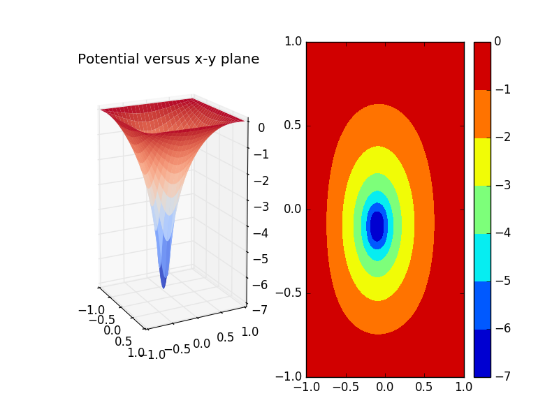
5.1 Potential with single charge(Jacobi Method)

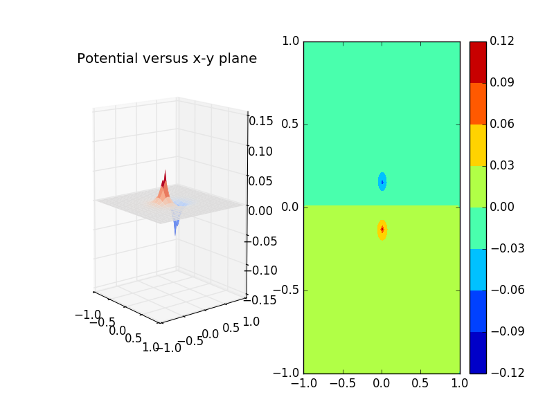
Now we set the unit charge at sites(50,50),and plot the potential versue(x-y) plane.

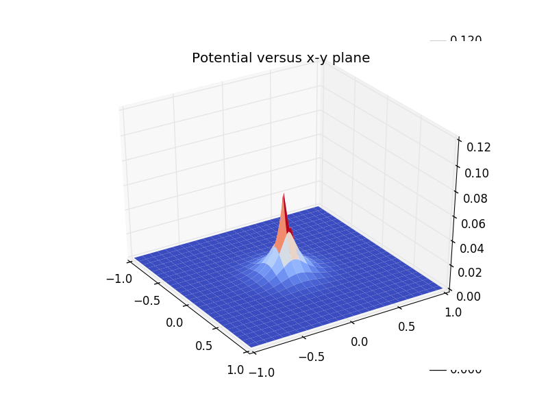
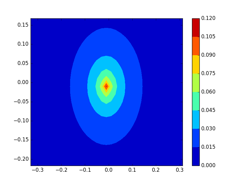
Next are the plot with distribution of potentials in 2D plane.That is the form of Coulomb's law! We now know the power of the numerrical mathod. Actually we can apply this method to more complicated systems where analytical ways can not work.

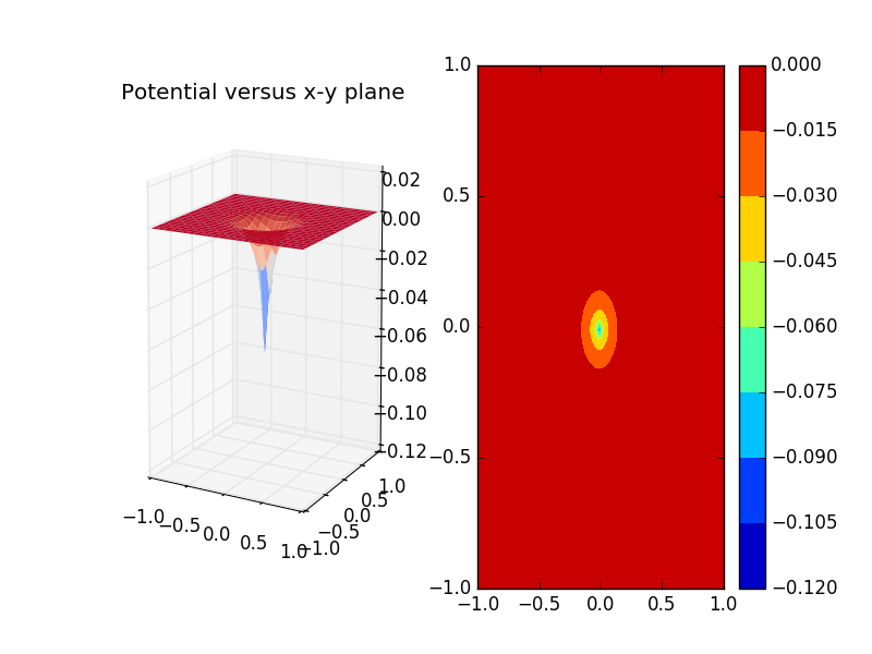
Now we set q=-1,we obtain his figurs.Its and reversed edition of q=1,obviously.

What if we set the area of $[40,60]\times[40,60]$ all to be negative charges?

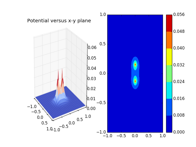
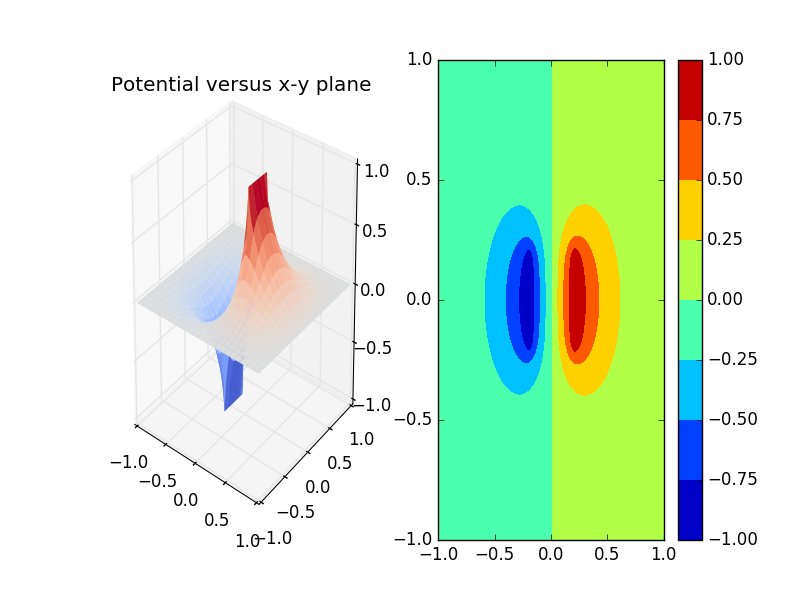
Two positive charge seperated by a distance.

Simulated plot:

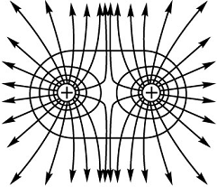
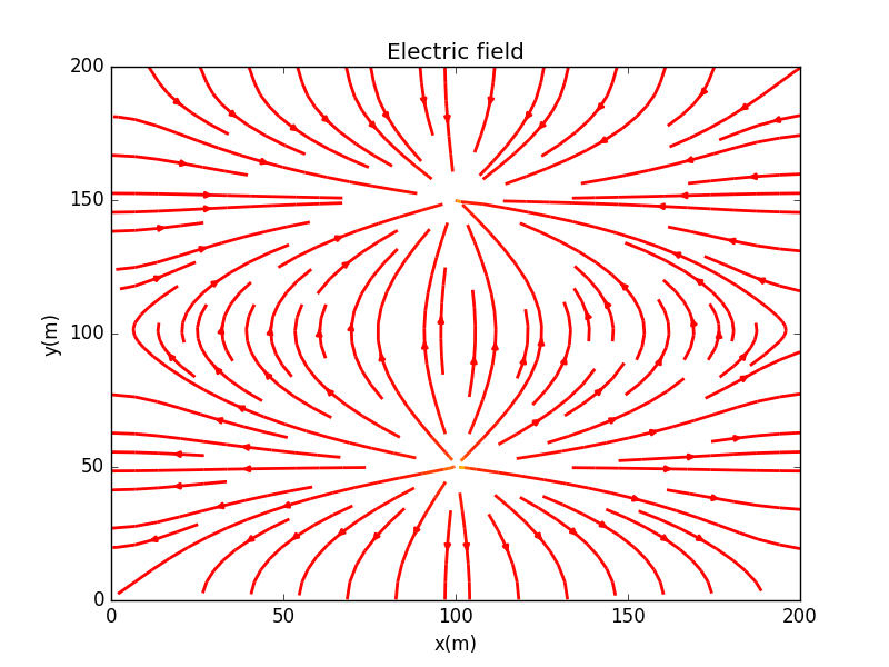
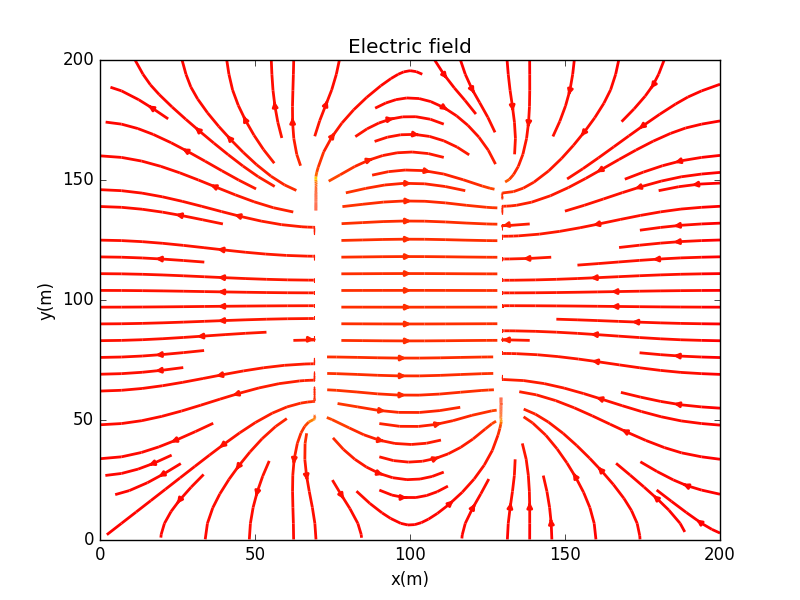
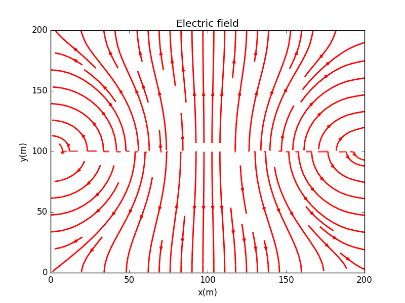
Next will be the electric field line between two repelling charge.

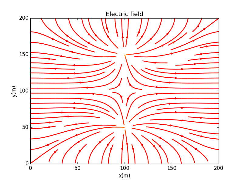
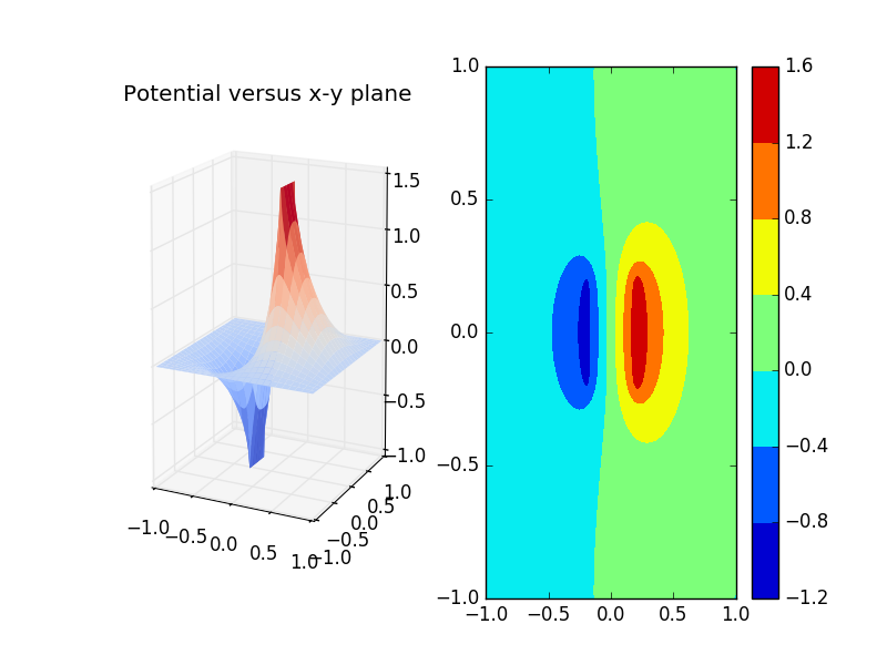
Two attractive points charge seperated by a distance

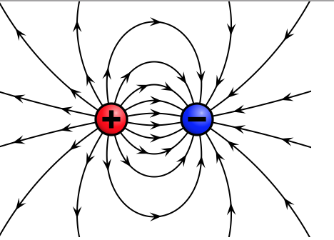
Simulated plot:

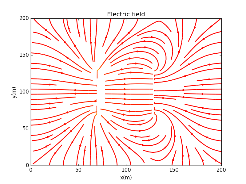
Here are the electric field lines of two attractive charges.

Now we change one of the charge to be $1.5$,and the other remains to be $1$,we will see the plot has already displayed evident insymmetry.

5.2 Potential for capacitor plates

Here we plot the two parallel capaciotor with $V=1$ and $V=-1$.It is pretty symmetry and applies to the realistic situation pretty well.As the array we chosed is relatively big, so we obtained a smoth counter plot, where different color stand for different value of potential. Look pretty beautiful! Now we know the poential distribution of the capacitor system.

What the electric fields line has just told us is that the electric filed between two parallel plates are almost uniform,which corresponds to our preceding expectation.

Now we change one of the capacitor from $V=1$ to $V=1.5$.In this figure, we are able to observe obvoulsy shift of the symmetry plot.

Here are the electric field plot.What is obvious to us is that the field lines are no longer symmetric at all due to the $V=1.5$v Capacitor plates versus $V=1.0$v

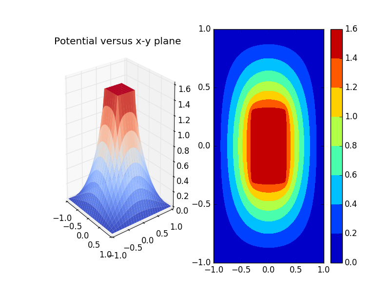
5.3 Potential for prism

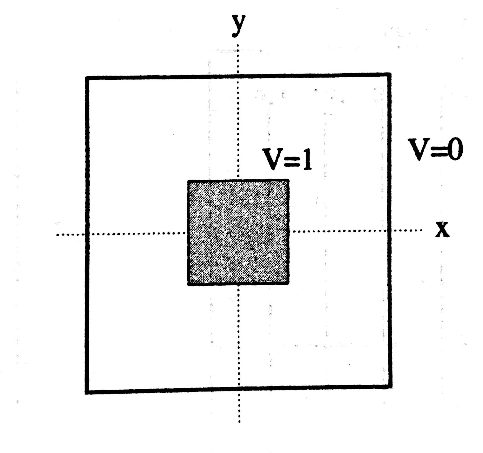
Schematic cross-section of a hollow metallic prism with a solid metallic inner conductor.The prism and inner conductor are persumed to be infinite in extend along z.The inner conductors are held at $V=1$ and the walls of the prism at $V=0$

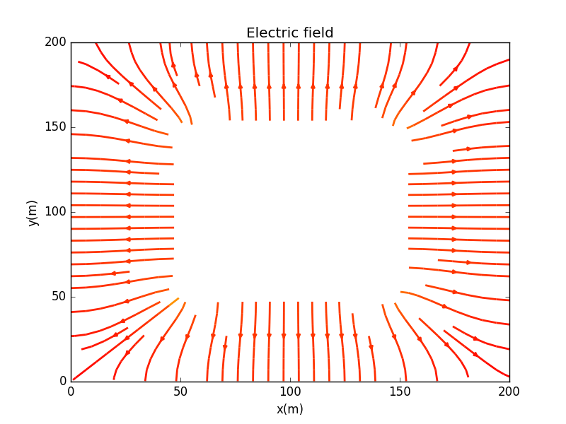
Here are the electric fields line,which shows that inside the conductors,there is no electric field,which leads to the conclusion that the conductors are equal-potential body.

5.4 A lighting rod

With the limitation of grid,we only set the leght of the chaged rod from $x=0$ to $x=99$.

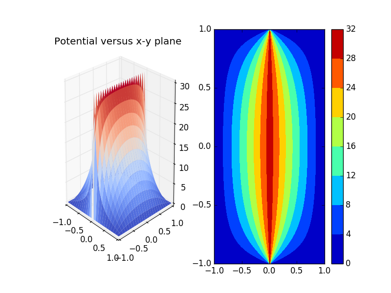
Electric fields line：

6 Acknowledge

1.Wikipedia, the free encyclopedia
2.Computational Physics,Nicholas J.Giordano,Hisao Nakanishi,the second edition,2006.
3.Electric Field-Wikipedia, the free encyclopedia