The Homework of Chapter Three

Author： 宗玥 2014301020004

Statistical-and-Thermal-Physics

---

Problem 3.2. Piggy bank

A piggy bank contains one penny, one nickel, one dime, and one quarter. It is shaken until two coins fall out at random. What is the probability that at least $0.30 falls out?

As we know one penny is 1 cent, one nickel is 5 cent, one dime worth 10 cent, one quater worth 25 cent. If we want to get 0.3 dollar, we need to get one nickel and one quater. So the probabilty is $\frac{1}{12}$

Problem 3.4. Free throws

A person hits 16 free throws out of 25 attempts. What is the probability that this person will make a free throw on the next attempt?

The probability is $16/25$

Problem 3.6. What’s in your purse?

A coin is taken at random from a purse that contains one penny, two nickels, four dimes, and three quarters. If x equals the value of the coin, find the average value of x.

As we know one penny is 1 cent, one nickel is 5 cent, one dime worth 10 cent, one quater worth 25 cent.
So $\overline x=\frac{1+2*5+4*10+3*25}{1+2+4+3}=12.6$
That means the average value of x is 12.6 cent equals $0.126

Problem 3.8. Choices

Suppose that you are offered the following choice:
(a) A prize of 50 dollars, or
(b) you flip a (fair) coin and win 100 dollars if you get a head, but $0 if you get a tail.
Which choice would you make? Explain your reasoning. Would your choice change if the prize was 40 dollars?

I will choose a prize of 50 dollars. Because it means I will get money 100%, and I won't change my choice when the prize was 40 dollars.

Problem 3.10. Thinking about probability

(a) Suppose that you were to judge an event to be 99.9999% probable. Would you be willing to bet 999999 dollars against 1 dollar that the event would occur? Discuss why probability assessments should be kept separate from decision issues.

(a) Even though the probabilty is 99.9999% but that doesn't mean the event must happen, and if it doesn't happen you will loss 999999 dollars. It is unworthy. We should keep probability assessments separate from decision issues. Because even though the probability is large enough, but it doesn't mean it can happen 100%, and if you can't suffer the ending then please let it go.

(b) In one version of the lottery the player chooses six numbers from 1 through 49. The player wins only if there is an exact match with the numbers that are randomly generated. Suppose that someone gives you a dollar to play the lottery. What sequence of six numbers between 1 and 49 would you choose? Are some choices better than others?

(b) I will choose some special number for me. Because the ending is totlaly random, and I don't have better choices.

(c) Suppose you toss a coin six times and obtain heads each time. Estimate the probability that you will obtain heads on your seventh toss. Now imagine tossing the coin 60 times, and obtaining heads each time. What do you think would happen on the next toss?

(c) In the first condition I will think that the probability is just larger than 50%. In the second condition, I will believe that the next toss will obtaine head.

(d) What is the probability that it will rain tomorrow? What is the probability that the Dow Jones industrial average will increase tomorrow?

(d) According to the weather report the probabilty that it will rain tomorrow is 11%, the probability that the Dow Jones industrial average will increase tomorrow is

(e) Give several examples of the use of probability in everyday life. In each case discuss how you would estimate the probability.

(e) In weather report, we use probability to predict the weather of tomorrow. In this condition we always through the data gathered by meteorological station and satellite.
When we make some decision in business such as the nature and quantity of the goods we need. In this condition we always do some surveys.

Problem 3.12. Rolling the dice

If a person rolls two dice, what is the probability P(n) of getting the sum n? Plot P(n) as a function of n.

We can get below：

n	P(n)
2	$\frac{1}{36}$
3	$\frac{1}{18}$
4	$\frac{1}{12}$
5	$\frac{1}{9}$
6	$\frac{5}{36}$
7	$\frac{1}{6}$
8	$\frac{5}{36}$
9	$\frac{1}{9}$
10	$\frac{1}{12}$
11	$\frac{1}{18}$
12	$\frac{1}{36}$

Then

$$P(n)=\left\{ \begin{array}{rcl} &\frac{n-1}{36}&,&2\le n\le7 \\ &\frac{13-n}{36}&,&7<n\le12 \\ \end{array} \right.$$

Problem 3.14. Rolling three dice

Suppose that three dice are thrown at the same time. What is the ratio of the probabilities that the sum of the three faces is 10 compared to 9?

If we throw three dice at the same time,
the probability that sum of the three faces is 10 equals $\frac{27}{216}=\frac{1}{8}$
the probability that sum of the three faces is 9 equals $\frac{25}{216}$.
So the ratio is $\frac{27}{25}$

Problem 3.16.

Show that, if $c$ is a constant, then

$$\overline{cf(x)} = c\overline{f(x)}　　　 (3.16)$$

$$\begin{eqnarray*} \overline{cf(x)}&=&\frac{\int_a^b cf(x)}{b-a}\\ &=&c \frac{\int_a^b f(x)}{b-a}\\ &=&c\overline{f(x)} \end{eqnarray*}$$

Problem 3.18. A couple with two children

(a) A couple has two children. What is the probability that at least one child is a girl?

(a) The probability that at least one child is a girl equals $\frac{3}{4}$

(b) Suppose that you know that at least one child is a girl. What is the probability that both children are girls?

(b) $\frac12$

(c) Instead suppose that we know that the oldest child is a girl. What is the probability that the youngest is a girl?

(c) $\frac12$

Problem 3.20. Uncertainty

(a) Consider the toss of a coin for which P1 = P2 = 1/2 for the two outcomes. What is the uncertainty in this case?

(a) $S=ln\Omega=ln2$

(b) What is the uncertainty for P1 = 1/5 and P2 = 4/5? How does the uncertainty in this case compare to that in part (a)?

(b) $S=-\sum_i P_ilnP_i=-\frac{1}{5}ln\frac{1}{5}-\frac{4}{5}ln\frac{4}{5}\approx0.5$

(c) On page 118 we discussed four experiments with various outcomes. Compare the uncertainty S of the third and fourth experiments.

(c) The third experiment:

$$S=ln4$$
The fourth experiment:
$$S=ln6$$

Problem 3.28. Coin flips

The outcome of N coins is identical to N noninteracting spins, if we associate the number of coins with N, the number of heads with n, and the number of tails with N − n. For a fair coin the probability p of a head is p = 1 2 and the probability of a tail is q = 1 − p = 1 2. What is the probability that in three tosses of a coin, there will be two heads?

$$P=\lgroup_3^2\rgroup p^2q=3*(\frac12)^3=\frac38$$

Problem 3.30. Binomial distribution

(a) Calculate the probability PN(n) that n spins are up out of a total of N for N = 4 and N = 16 and put your results in a table. Calculate the mean values of n and n2 using your tabulated values of PN(n). It is possible to do the calculation for general p and q, but choose p = q = 1/2 for simplicity. Although it is better to first do the calculation of PN(n) by hand, you can use Program Binomial.

(a) If N=4

$$\begin{eqnarray*} P_4(n)&=&\lgroup_4^n \rgroup p^n q^{4-n}\\ &=&\frac{24}{n!(4-n)!}p^nq^{4-n}\\ &=&\frac{24}{n!(4-n)!}\frac{1}{2^4}\\ &=&\frac{3}{2n!(4-n)!}\\ \overline n&=&\sum_{n=0}^4 \frac{3n}{2n!(4-n)!}\\ &=&\frac{3*0+12*1+18*2+12*3+3*4}{48}\\ &=&2\\ \overline{n^2}&=&\sum_{n=0}^4 \frac{3n^2}{2n!(4-n)!}\\ &=&\frac{3*0+12*1+18*4+12*9+3*16}{48}\\ &=&5 \end{eqnarray*}$$
If N=16
$$\begin{eqnarray*} P_{16}(n)&=&\lgroup_{16}^n \rgroup p^n q^{16-n}\\ &=&\frac{16!}{n!(16-n)!}p^nq^{16-n}\\ &=&\frac{16!}{2^{16}n!(16-n)!}\\ \overline n&=&\sum_{n=0}^{16}\frac{16!n}{2^{16}n!(16-n)!}\\ &=&Np\\ &=&8\\ \overline {n^2}&=&\sum_{n=0}^{16}\frac{16!n^2}{2^{16}n!(16-n)!}\\ \end{eqnarray*}$$
However for binomial distribution we have $Vax(n)=Npq$
So the mean value of $n^2$ equals $Vax(n)+\overline n^2=68$

(b) Use Program Binomial to plot PN(n) for larger values of N. Assume that p = q = 1/2. Determine the value of n corresponding to the maximum of the probability and visually estimate the width for each value of N. What is your measure of the width? One measure is the value of n at which PN(n) is equal to half its value at its maximum. What is the qualitative dependence of the width on N? Also compare the relative heights of the maximum of PN for increasing values of N.

(b)

(c) Program Binomial also plots PN(n) versus n/n. Does the width of PN(n) appear to become larger or smaller as N is increased?

(c)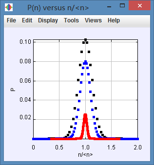
We can get that the width of $P_N(n)$ appear to become smaller as N is increased.

(d) Plot lnPN(n) versus n for N = 16. (Choose Log Axes under the Views menu.) Describe the qualitative dependence of lnPN(n) on n. Can lnPN(n) be fitted to a parabola of the form A + B(n−n)2, where A and B are fit parameters?

(d)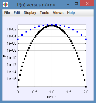
The blue line is the ending of N=16.

Problem 3.32. Width of the binomial distribution

Compare the calculated values of σn from (3.99) with your estimates in Problem 3.30 and to the exact result (3.82) for N = 4. Explain why σn is a measure of the width of PN(n).

In program 3.30, when $N=4$, $\overline n=2, \overline {n^2}=5$,so $\overline{n^2}-(\overline n)^2=1$.According to (3.99),we have $\sigma_n=Npq=1$.The result is equal. When $N=16$, we will get the same conclusion.
We can discover from the picture that most of the point gather in interval $[\mu-3\sigma,\mu+3\sigma]$. So a large $\sigma$ means the width is large.

Problem 3.34. Density fluctuations

(a) What is the probability p that a particular molecule is in the volume V1?

(a) $p=\frac{V_1}{V}$

(b) What is the probability that N1 molecules are in V1 and N2 molecules are in V2, where N = N1 + N2?

(b)

$$\begin{eqnarray*} P&=&\lgroup^{N_1}_{N}\rgroup p^{N_1}(1-p)^{N_2}\\ &=&\frac{N!}{N_1!N_2!}(\frac{V_1}{V})^{N_1}(\frac{V_2}{V})^{N_2} \end{eqnarray*}$$

(c) What is the average number of molecules in each part?

(c) $\overline{N_1}=Np=\frac{NV_1}{V}$

(d) What are the relative fluctuations of the number of molecules in each part?

(d) $\sigma_{N_1}=\sqrt{p(1-p)N}=\sqrt{\frac{V_1V_2N}{V^2}}$
　$\sigma_{N_2}=\sqrt{(1-p)pN}=\sqrt{\frac{V_1V_2N}{V^2}}$
　

Problem 3.36. Monte Carlo simulation of a one-dimensional random walk

(a) Is the value of x for one trial of any interest? Why do we have to average over many trials?

(a) No, it isn't. Because just one trial has too much uncertainty. That is why we need to average over many trials.

(b) Will we obtain the exact result for the probability distribution by doing a Monte Carlo simulation?

(b) No we won't. Monte Carlo simulation just show us the ending of caculation which is not the exact result for the probability distribution.

(c) Describe the changes of the histogram for larger values of N and p = 1/2.

(c) While N is small, such as N=16, we get below:

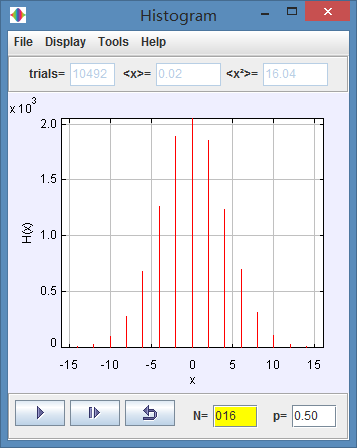
However when we set N=1600, we will get:

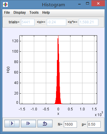
We can get that the width of the histogram for large values of N and p=1/2 is much smaller than that of small values of N.

(d) What is the most probable value of x for p = 1/2 and N = 16 and N = 32? What is the approximate width of the distribution? Estimate the width visually. One way to do so is to determine the value of x at which the value of the histogram is one-half of its maximum value. How does the width change as a function of N for fixed p?

(d) The most probable value of x in the two situation is 0.

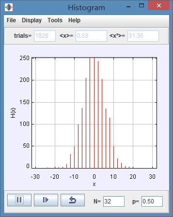
We can compare these histograms and get the width of N=16 is about 30. For N=32, the width is about 40. Even though through these two histogrames, the width is increased. When we comapre the ending between N=16 and 1600, we can get the width is decreased with the increasing of N.

(e) Choose N = 4 and p = 1/2. How does the histogram change, if at all, as the number of walks increases for fixed N?

(e)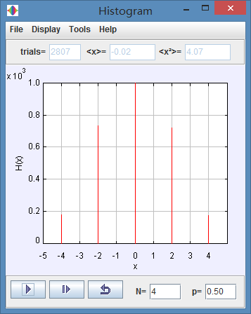
The X-axis coordinates are not changed, the y-axis coordinates are increasing with time goes by.

Problem 3.38. Simulation of a one-dimensional random walk with variable step length +++++++

(a) The step length is generated at random with a uniform probability between 0 and 1. Calculate the mean displacement and its variance for one step.

(a)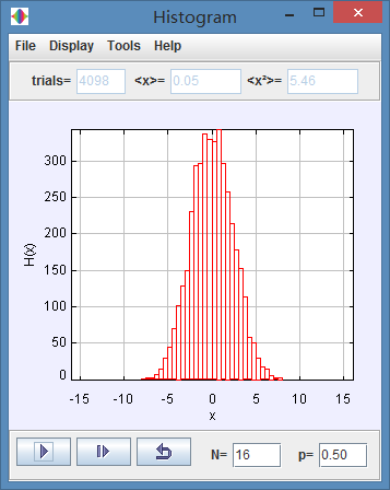
After long time the mean displacement is 0.05 the variance is 5.46.

(b) Compare your analytical results from part (a) to the results of the simulation for N = 1.

(b)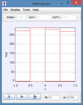
The mean displacement is 0, and the variance is 0.33.

(c) How does the variance of the displacement found in the simulation for N = 16 depend on the variance of the displacement for N = 1 that you calculated in part (a)?

(c) The variance of the displacement found in the simulation for N=16 is larger than that in the simulation for N=1.

(d) Explore how the histogram changes with the bin width. What is a reasonable choice of the bin width for N = 100?

(d)

Problem 3.40. Probability density for velocity

(a) Show that $p(v)$ is normalized. Use the fact that [see (A.15)]

$$\int_0^{\infty}e^{-au^2}du=\frac12\sqrt{\frac{\pi}{a}}　　(3.123)$$ Note that this calculation involves doing three similar integrals that can be evaluated separately.

(a)

$$\begin{eqnarray*} p(v)&=&\int_0^{\infty}\int_0^{2\pi}\int_{-\infty}^{+\infty}(\frac{a}{\pi})^{\frac32}e^{-av^2}v^2dvd\varphi sin\theta d\theta\\ &=&(\frac{a}{\pi})^{\frac32}\int_{-\infty}^{+\infty}e^{-av^2}v^2dv\int_0^{+\infty}sin\theta d\theta \int_0^{2\pi}d\varphi\\ &=&(\frac{a}{\pi})^{\frac32}*2*2\pi*\frac14(\frac{\pi}{a^3})^{\frac12}\\ &=&1 \end{eqnarray*}$$
So $p(v)$ is normalized.

(b) What is the probability that a particle has a velocity between vx and vx +dvx, vy and vy +dvy, and vz and vz + dvz?

(b)????

$$\begin{eqnarray*} P(v_x)&=&p(v_x)dv_x\\ P(v_y)&=&p(v_y)dv_y\\ P(v_z)&=&p(v_z)dv_z \end{eqnarray*}$$

(c) What is the probability that vx ≥0, vy ≥0, vz ≥ 0 simultaneously?

(c)

$$\begin{eqnarray*} P(v_x>0)&=&\int_0^{+\infty}p(v_x)dv_x\\ &=&\int_0^{+\infty}(\frac{a}{\pi})^{\frac32}e^{-av_x^2}dv_x\\ &=&\frac{a}{2\pi}\\ \end{eqnarray*}$$
$P(v_x>0)=P(v_y>0)=P(v_z>0)$
So, the probability that $v_x>0,v_y>0, v_z>0$simultaneously is $(\frac{a}{2\pi})^3$

Problem 3.42. Uniform probability distribution

(a) Sketch the dependence of p(x) on x.

(a)

(b) Find the first four moments of p(x).

(b)

(c) Calculate the value of the fourth-order cumulant C4 defined in (3.125) for the probability density in (3.126). Compare your result to the corresponding result for C4 for the Gaussian distribution.

(c)

$$\begin{eqnarray*} \overline x&=&\int xp(x)dx\\ &=&\int_{-a}^{a} \frac{x}{2a}dx\\ &=&0\\ \overline {x^2}&=&\int x^2p(x)dx\\ &=&\int_{-a}^{a}\frac{x^2}{2a}dx\\ &=&\frac{a^2}{3}\\ \overline{x^3}&=&0\\ \overline{x^4}&=&\int x^4 p(x)dx\\ &=&\int_{-a}^{a}\frac{x^4}{2a}dx\\ &=&\frac{a^4}{5}\\ \end{eqnarray*}$$
So we get
$$\begin{eqnarray*} C_4&=&\overline{x^4}-4\overline{x^3}\overline x-3\overline{x^2}^2+12\overline{x^2}\overline x^2-6\overline x^4\\ &=&\frac{a^4}{5}-0-3(\frac{a}{3})^2+0-6\frac{a^4}{5}\\ &=&-\frac{2a^4}{15} \end{eqnarray*}$$

Problem 3.44. Analysis of Figure 3.9

(a) Estimate the absolute width and the relative width ∆S/S of the distributions shown in Figure 3.9 for N = 100 and N = 800.

(a)

(b) Does the error of any one measurement of S decrease with increasing N as expected?

(b) Yes, it does.

(c) How would the plot change if the number of measurements M were increased to M = 100,000?

(c) The trend of the plot will not change but the point will get much closer.

Problem 3.46. Random walks and the central limit theorem

Use the central limit theorem to find the probability that a one-dimensional random walker has a displacement between x and x + dx. (There is no need to derive the central limit theorem.)

If we set the probability that the walker walk alonge +x axis is p, and we did this experiment n times, which A happens $n_A$ times.
Thus,

$$\begin{eqnarray*} p(\frac{n_A-np}{\sqrt{np(1-p)}}\le x)&=&\Phi(x)=\frac{1}{\sqrt{2\pi}}\int_{-\infty}^{x}e^{-\frac{t^2}{2}}dt\\ P(x\le n_a\le x+dx)&=&P(\frac{x-np}{\sqrt{np(1-p)}}\le \frac{n_A-np}{\sqrt{np(1-p)}}\le \frac{x+dx-np}{\sqrt{np(1-p)}})\\ &=&\Phi(\frac{x+dx-np}{\sqrt{np(1-p)}})-\Phi(\frac{x-np}{\sqrt{np(1-p)}}) \end{eqnarray*}$$

Problem 3.52. Characteristic function of a Gaussian

Calculate the characteristic function of the Gaussian probability density.

For Gaussian probability density, we have

$$f(x)=\frac{1}{\sqrt{2\pi}\sigma}e^{-\frac{(x-\mu)^2}{2\sigma^2}}$$
So the characteristic function of it is:
$$\begin{eqnarray*} \phi(k)&=&\int_{-\infty}^{\infty}e^{ikx}f(x)dx\\ &=&\int_{-\infty}^{\infty}e^{ikx}\frac{1}{\sqrt{2\pi}\sigma}e^{-\frac{(x-\mu)^2}{2\sigma^2}}dx\\ &=&\int_{-\infty}^{\infty}e^{ik(x-\mu)}e^{\mu}\frac{1}{\sqrt{2\pi}\sigma}e^{-\frac{(x-\mu)^2}{2\sigma^2}}dx\\ &=&\frac{1}{\sqrt{2\pi}\sigma}e^{\mu}\int_{-\infty}^{\infty}e^{ik(x-\mu)}e^{-\frac{(x-\mu)^2}{2\sigma^2}}d(x-\mu)\\ \end{eqnarray*}$$
If we set $x-\mu=y$，$\frac{1}{2\sigma^2}=a$
$$\begin{eqnarray*} \phi(k)&=&\frac{1}{\sqrt{2\pi}\sigma}e^{\mu}\int_{-\infty}^{\infty}e^{-(ay^2-iky)}dy\\ &=&\frac{1}{\sqrt{2\pi}\sigma}e^{\mu}\int_{-\infty}^{\infty}e^{-a(y-\frac{ik}{2a})^2+\frac{k^2}{4a}}dy\\ &=&\frac{1}{\sqrt{2\pi}\sigma}e^{\mu\frac{k^2}{4a}}\int_{-\infty}^{\infty}e^{-(\sqrt ay-\frac{ik}{2\sqrt a})^2}dy\\ &=&\frac{1}{\sqrt{2\pi}\sigma}e^{\mu\frac{k^2}{4a}}\int_{-\infty}^{\infty}e^{-u}\frac{1}{\sqrt a}du\\ &=&\frac{1}{\sqrt{2\pi}\sigma}e^{\mu\frac{k^2}{4a}}\sqrt{\frac{\pi}{a}}\\ &=&exp(\frac{\mu k^2}{4a}) \end{eqnarray*}$$