张梓桐计算物理第八次作业

1 Problem

Problem 3.18,3.20

2 Abstract

With the dicusssion the Euler method in calculating projectile movement of a cannon shell,in the passage,we are going to talk about the Euler-Cromer method of the better calculation of oscillatory under damped and external force.After we have calculated the Poincare Section of external force only at $F_D=1.2N$,now we turn to differnet situations of the various of $F_D$,in order to see the differnece and changes between them inside.

3 Background

Now we start to figure out the movement rule of a damped and forced pendulum.With the basic knowledge of Newtoon second law and the definition of $w$, we have the following equation:

$$\begin{eqnarray*} \frac{d^{2}\theta}{dt^{2}}=-\frac{g}{l}sin\theta-q\frac{d\theta}{dt}+F_{D}sin(\Omega_Dt) \end{eqnarray*}$$
where $F_{D}$ is the module of the external force with $SI$ unit,and $\Omega_{D}$ is the frequency of external force,also with $SI$ unit.
Here we introduce the variables $w$ to transfer the secdonary differential equation into firs-order differential equation:
$$\begin{eqnarray*} \frac{dw}{dt}=-\frac{g}{l}sin\theta-q\frac{d\theta}{dt}+F_{D}sin(\Omega_Dt) \end{eqnarray*}$$
$$\begin{eqnarray*} \frac{d\theta}{dt}=w \end{eqnarray*}$$
Now we rewrite the physics formula into precodes,notcing the Euler-Cromer method,rather than Euler method,which will lead to a divergence in the infinity.

• For each time step $i$,calculate $w$ and $\theta$ at time step $i+1$.

• $w_{i+1}=w_{i}-[\frac{g}{l}sin\theta_{i}+qw_{i}-F_{D}sin(\Omega_Dt)]\Delta t$

• $\theta_{i+1}=\theta_{i}+w_{i+1}\Delta t$

• If $\theta_{i+1}$ is out of the $[-\pi,+\pi]$,add or substract $2\pi$ to keep it in this range.

• $t_{i+1}=t_{i}+\Delta t$

• Repeat for the deisred number of time steps.

All above is just simple backgrounds of the problem.Here we are going to talk about the way to construct the bifurcation figure.

• For each value of $F_D$ we have calculated $\theta$ as a function of time.

• After waiting for 300 driving periods so that the intial transients have decayed away.

• We plot $\theta$ at times that were in phase with the driving force as a function of $F_D$

4 Main body

Program to calculate the Ponicare Section is no longer needed to be illustrated ,you can refer to my last assignment.
Here are program to draw the Bifurcation plot:

import math
import pylab as pl
import numpy as np
class oscillatory_motion:
    def __init__(self,Fd=1.2,OmegaD=2./3,q=0.5,intial_theta=0.2,intial_omega=0,time=1000,step=1000):
        self.Fd=Fd
        self.OmegaD=OmegaD
        self.intial_theta=intial_theta
        self.intial_omega=intial_omega
        self.step=step
        self.cycle=2*math.pi/OmegaD
        self.dt=self.cycle/step
        self.time=time
        self.Theta=[self.intial_theta]
        self.originTheta=[self.intial_theta]
        self.Omega=[self.intial_omega]
        self.Time=[0]
        self.q=q
    def run(self):
        while self.Time[-1]<self.time:
            tmp_Omega=self.Omega[-1]+(-math.sin(self.Theta[-1])-self.q*self.Omega[-1]+self.Fd*math.sin(self.OmegaD*self.Time[-1]))*self.dt
            self.Omega.append(tmp_Omega)
            tmp_Theta=self.Theta[-1]+tmp_Omega*self.dt
            self.originTheta.append(tmp_Theta)
            while tmp_Theta<-math.pi:
                tmp_Theta=tmp_Theta+2*math.pi
            while tmp_Theta>math.pi:
                tmp_Theta=tmp_Theta-2*math.pi
            self.Theta.append(tmp_Theta)
            tmp_Time=self.Time[-1]+self.dt
            self.Time.append(tmp_Time)  

Above are the general program to do calculation.
Next will be the addtional section for Bifuraction Plot.

#This section is used to caluclate and store the data of theta after 300 periods of driving foce and a fixed driving force
def Bifurcation_Plot(init_NUMBER=0,F_D=1.2,frequency=2./3,friction=0.5,color='black',slogan=''):
    tmp_variable=oscillatory_motion(Fd=F_D,OmegaD=frequency,q=friction,time=400*2*math.pi/frequency,)
    tmp_variable.run()
    Theta=[]
    for i in range(100):
        Theta.append(tmp_variable.Theta[(300+i+init_NUMBER)*tmp_variable.step])
    Fd=[F_D]*len(Theta)   
    return (Fd,Theta)

Here are the order to possess:

#Set the intial F_D to be 1.35 and with a interval of 0.001, end with F_D =1.5,other situation can be adapted from this origin program as you wish
tmp_FD=[]
tmp_theta=[]
for i in np.arange(1.35,1.5,0.001):
    a=Bifurcation_Plot(F_D=i,frequency=2./3)
    tmp_FD.extend(a[0])
    tmp_theta.extend(a[1])
pl.scatter(tmp_FD,tmp_theta,s=0.1,label=r'$\Omega_D=2/3$')
pl.legend()

5 Results

5.1 Part 1

Firstly let's take a glimpse of $F_D=1.2N$ situation.

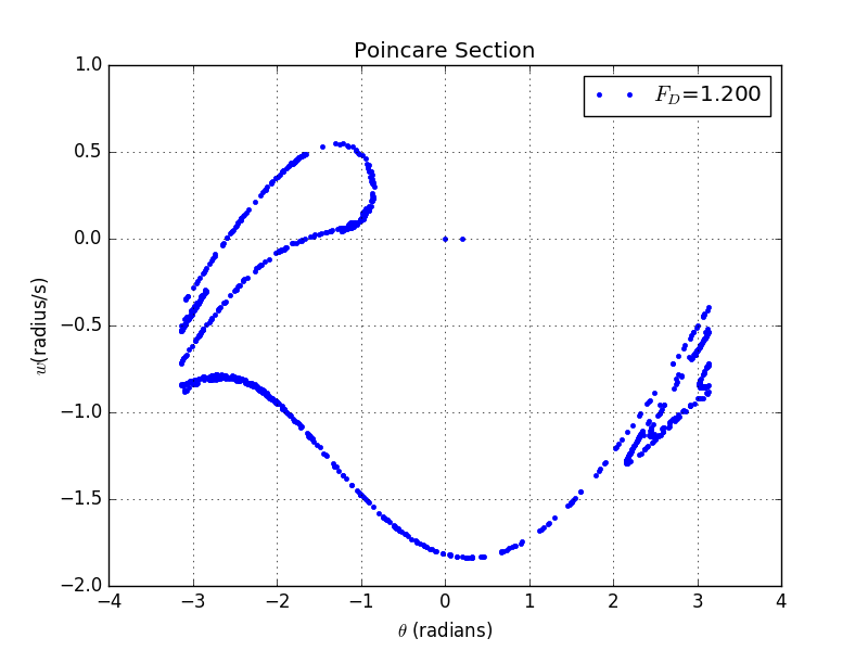
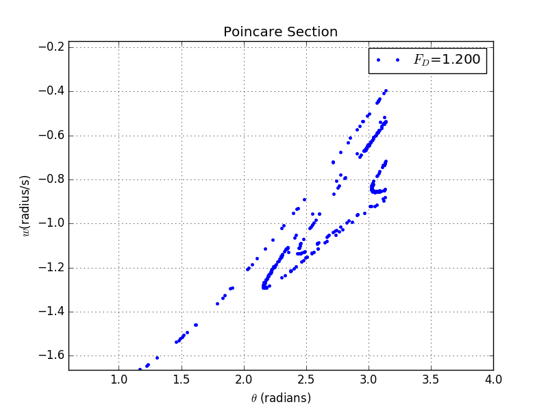
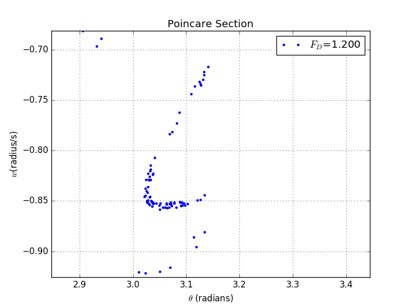
And here are the details of the plot:

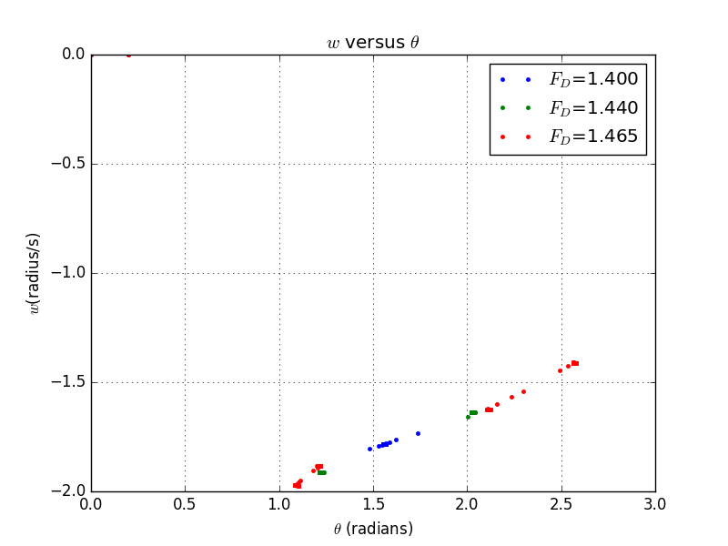
Secondly,Let's look at the differnent time choosing for in-phase to $\frac{\pi}{4}$ out of phase and $\frac{\pi}{2}$ out of phase:

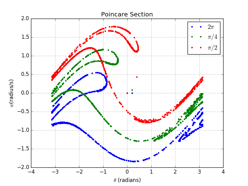
Thirdly,we are going to show the Poincare Plot for various $F_D$
This plot contains $F_D=1.4N$,$F_D=1.44N$,$F_D=1.465N$

5.2 Part 2

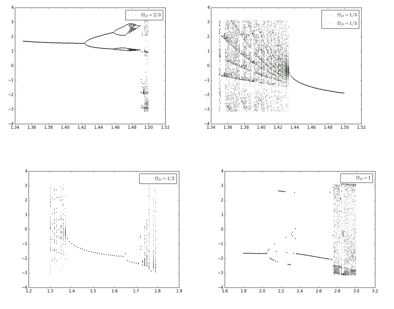
Now we'd like to talk about the Bifuration figure:
We choose the $\Omega_D=\frac{2}{3}$ and $q=0.5$

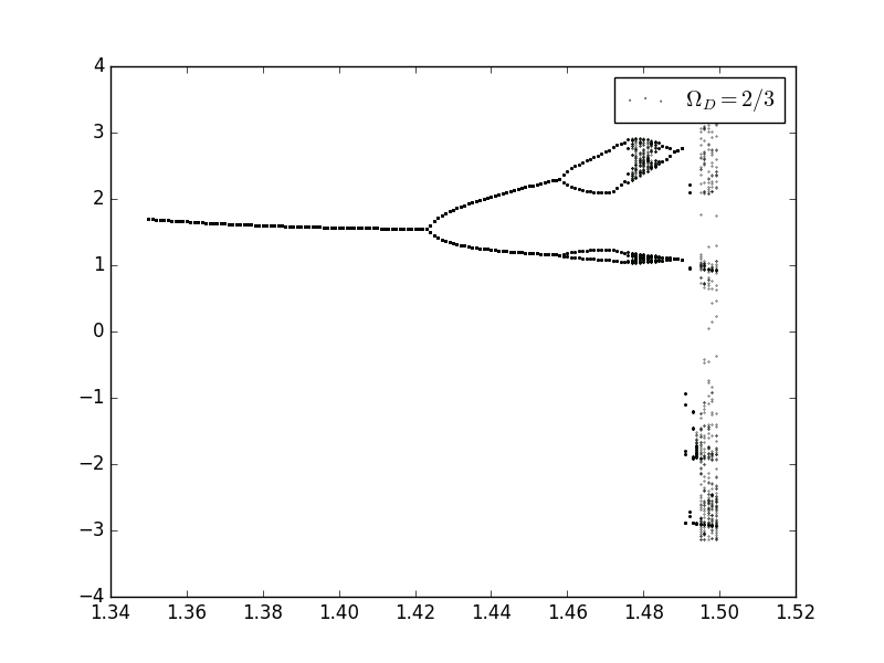
Next are some details:

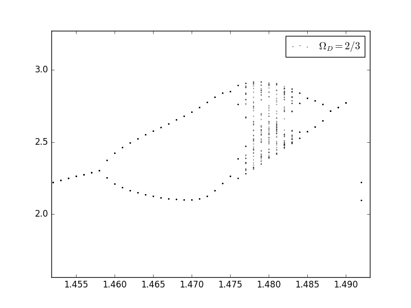
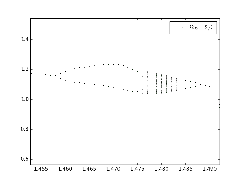
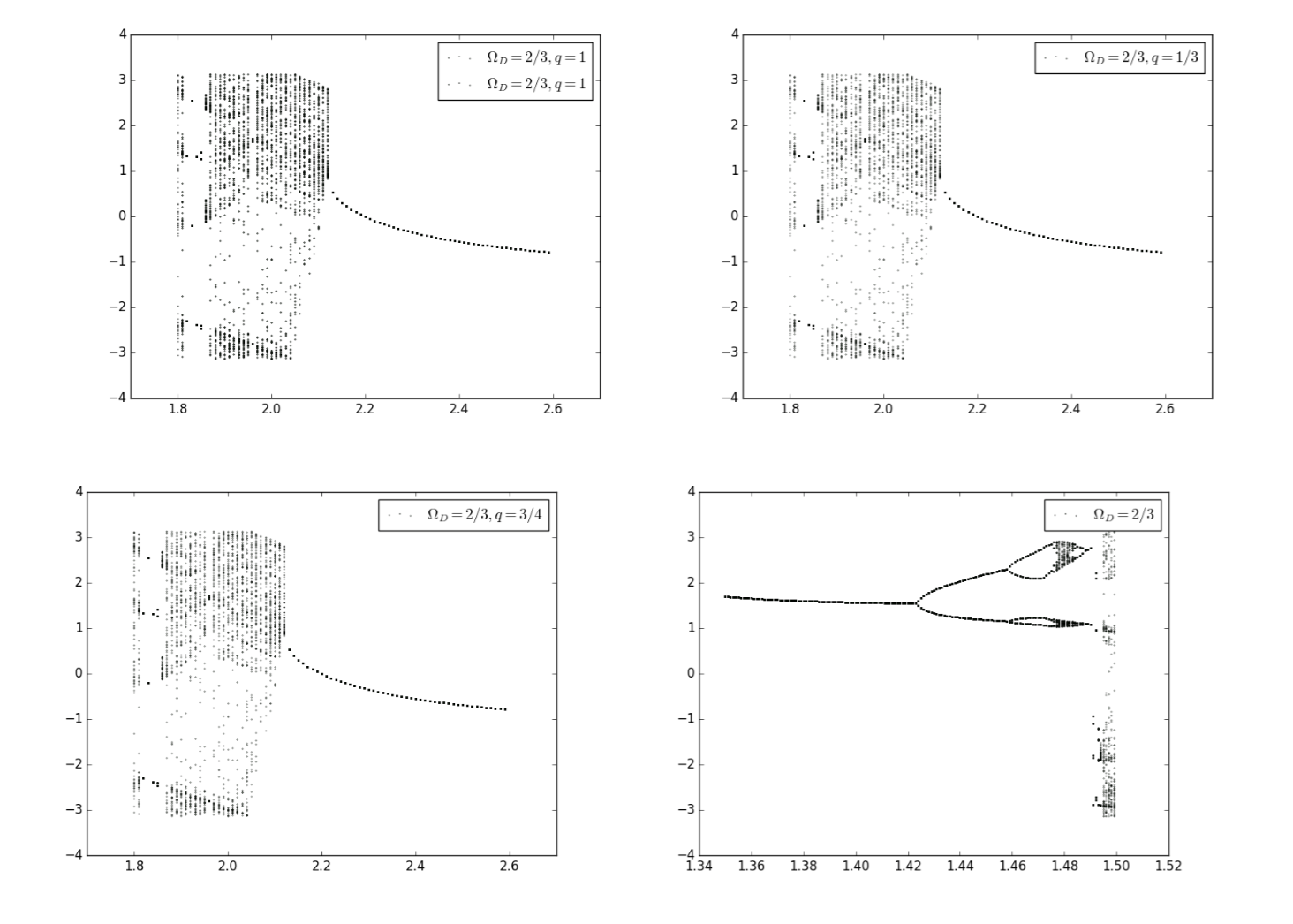
Here are the plots with different $\Omega_D$

Now we change the fricition factor $q$ to $\frac{1}{3},\frac{2}{3},\frac{1}{2},1$

6 Vpython display

For this part the source code is(a definition in the oscillatory_motion class)

from __future__ import division
from visual import *
from math import *

q=0.5
l=9.8
g=9.8
f=2/3
dt=0.04
theta0=0.2
omega0=0
ceil=box(pos=(0,5,0),size=(5,0.5,2),material=materials.bricks)
ball=sphere(pos=(l*sin(theta0),5-l*cos(theta0),0),radius=1,material=materials.emissive,color=color.green)
ball.omega=omega0
ball.theta=theta0
ball.t=0
ball.F=0.5
string=curve(pos=[ceil.pos,ball.pos],color=color.yellow)
po=arrow(pos=ball.pos,axis=(10*ball.omega*cos(ball.theta),10*ball.omega*sin(ball.theta),0),color=color.yellow)
while True:
    rate(100)
    ball.omega=ball.omega-((g/l)*sin(ball.theta)+q*ball.omega-ball.F*sin(f*ball.t))*dt
    angle_new=ball.theta+ball.omega*dt
    while angle_new>pi:
        angle_new-=2*pi
    while angle_new<-pi:
        angle_new+=2*pi
    ball.theta=angle_new
    ball.pos=(l*sin(ball.theta),5-l*cos(ball.theta),0)
    string.pos=[ceil.pos,ball.pos]
    po.pos=ball.pos
    po.axis=(10*ball.omega*cos(ball.theta),10*ball.omega*sin(ball.theta),0)
    ball.t=ball.t+dt

6.1 GIF 1

Here are the gif for this code($F_D=0.5N$):
There is barely chaos for low $F_D$

6.2 GIF 2

Here are the gif for this code($F_D=1.2N$):
You can see obviously chaos in this gif

7 Thanks

1.Wang shixing for his frame of program
2.Wu yuqiao for his frame of Vpython program
3.LATEX