@fanxy
2020-03-15T08:52:43.000000Z
字数 8850
阅读 7233
第三讲 数据可视化与编程基础
樊潇彦 复旦大学经济学院 金融数据
0. 准备工作
下载 Ch03.rar,解压缩后存于工作目录下。
setwd("D:\\...\\Ch03") # 设定工作目录,注意为/或\\rm(list=ls()) # 清内存## 调用之前已安装且当前要用的包library(tidyverse)library(readstata13)library(haven)library(readxl)## 安装和调用本节要用的包install.packages(c("ggplot2","ggvis","shiny","dygraphs"))library(ggplot2)library(ggvis)library(shiny)library(dygraphs)
1. 数据可视化
1.1 基础作图
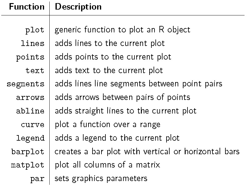
# 基础绘图 plot,包括 points, lines, scatter, histogram等data(iris)plot(iris$Sepal.Length) # 单变量点图plot(iris$Sepal.Length,type="l") # 单变量线图plot(x=iris$Sepal.Length, y=iris$Petal.Length) # 双变量散点图plot(x=iris$Sepal.Length, y=iris$Petal.Length, type="h") # 双变量柱状图plot(x=iris$Species, y=iris$Petal.Length, type="h") # 连续变量按离散变量分组的箱式图# 条形图 barplotmsft <- c(26.85,27.41,28.21,32.64,34.66,34.30,31.62,33.40)msft.returns <- msft[-1] / msft[-length(msft)] - 1names(msft.returns) <- month.abb[1:length(msft.returns)]barplot(msft.returns, col="blue")barplot(msft.returns, names.arg=month.name[1:length(msft.returns)],col="blue",las=2)# 饼图 piex <-1:5;pie(x,col=rainbow(5))box()# 向日葵图 sunflowerplotsunflowerplot(iris[,3:4])# 绘制矩阵或数据框的二元图 pairsdata(iris)pairs(iris[1:4], main = "Anderson's Iris Data -- 3 species",pch = 21,bg = c("red", "green3", "blue")[unclass(iris$Species)])# 多个数据作图 matplotset.seed(1)x <- cumsum(rnorm(50))y <- cumsum(rnorm(50))z <- cumsum(rnorm(50))matplot(cbind(x,y,z),col=2:4,type="l",lty=1, xlab="", ylab="")legend("bottom",legend=c("x","y","z"),lty=1,col=2:4,bty="n")# 根据指定函数绘制指定范围的曲线图curve(sin, -2*pi, 2*pi, xname = "t")
1.2 修饰和保存
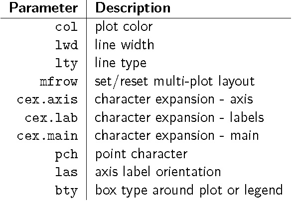
# 以参数`par`和标签`legend`为例:intc <- c(20.42,20.48,21.43,23.50,24.04,24.00,23.11,21.98)intc.returns <- intc[-1] / intc[-length(intc)] - 1barplot(rbind(msft.returns,intc.returns),beside=T,col=c(2,4))legend(x="topleft",legend=c("MSFT","INTC"),pch=15,col=c(2,4),bty="n")# 生成一个绘图窗口在其中绘制图形后用savePlot()函数保存windows()plot(1:10)rect(1, 5, 3, 7, col="blue")savePlot("test01", type="jpg",device=dev.cur(),restoreConsole=TRUE)# 直接在jpeg设备上绘制图形,完成后使用dev.off()关闭设备,存盘退出jpeg(file="myplot.jpeg")plot(1:10)rect(1, 5, 3, 7, col="blue")dev.off()
1.3 ggplot2
Basic Components of a ggplot2 Plot
- A data frame
- aesthetic mappings: how data are mapped to color, size and shapes
- geoms: geometric objects like points, lines, histograms, etc.
- stats: statistical transformations like binning, quantiles, smoothing.
- facets: for conditional plots.
- scales: what scale an aesthetic map uses (example: male = red, female = blue).
- coordinate system
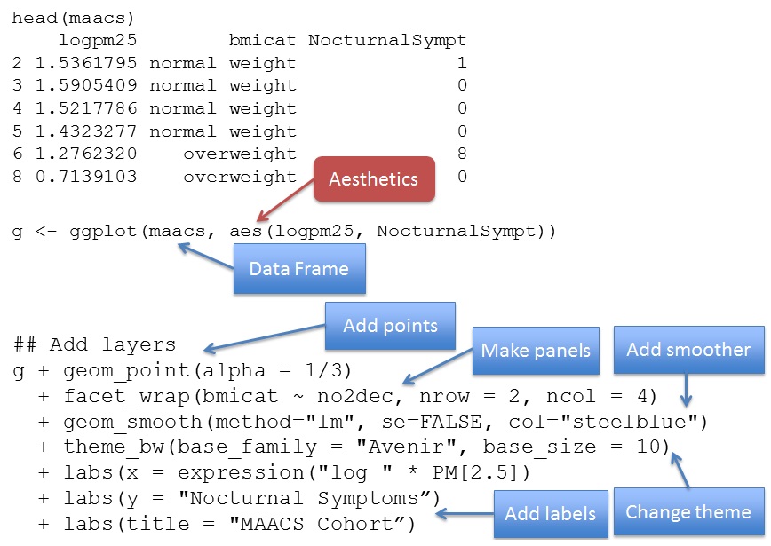

library(ggplot2)data(diamonds) # 调用钻石数据set.seed(42) # 设随机数,抽1000个样本small <- diamonds[sample(nrow(diamonds), 1000), ]head(small)# 生成空白图,查看ggplot对象要素p = ggplot()class(p)names(p)# 数据和映射# 以克拉(carat)、切工(cut)、透明度(clarity)等因素对钻石价格(price)的影响为例:ggplot(data = small,mapping = aes(x = carat, y = price, # 纵横轴color = cut, shape = clarity)) +geom_point()# 几何与统计ggplot(small) +geom_density(aes(x=price, colour=cut))# 分面与标签ggplot(small, aes(x=carat, y=price, color=color))+ # 标题、纵横轴标签geom_point() +facet_wrap(~cut) + # 一页多图labs(title ="Diamonds", x = "Carat", y = "Price") +theme_bw()
1.4 ggvis
1.主要命令
library(ggvis)library(dplyr)data(mtcars)# 散点和拟合线:points, smoothsmtcars %>%ggvis(~wt, ~mpg) %>%layer_points(fill= ~factor(cyl))%>% # 除填充(fill)外,还可设边界(stroke)、大小(size)、形状(shape)和透明度(opacity)layer_lines(stroke:= "gray") %>%layer_smooths()# 线和条:lines, barsdata(pressure)pressure %>%ggvis(~temperature, ~pressure) %>%layer_lines(stroke := "red") %>%layer_bars(width=20, fill:=NA)
2.统计作图
# Boxplotsmtcars %>%ggvis(~factor(cyl), ~mpg) %>%layer_boxplots()# Histogramscocaine %>%ggvis(~potency) %>%layer_histograms(width = 10, center = 0, fill := "pink") %>%add_axis("x", title = "potency") %>%add_axis("y", title = "histograms")# Densitiescocaine %>%ggvis(~potency) %>%layer_densities(fill := NA, stroke := "red") %>%add_axis("x", title = "potency") %>%add_axis("y", title = "densities")
3.回归预测
mtcars %>%ggvis(~wt, ~mpg) %>%layer_points() %>%layer_smooths() %>%layer_model_predictions(stroke := "red", model = "lm", se = TRUE)mtcars %>%ggvis(~wt, ~mpg, fill = ~factor(cyl)) %>%layer_points() %>%group_by(cyl) %>% # 分组回归layer_model_predictions(model = "lm")
4.交互式作图
- input_slider:滑块
- input_checkbox:一个复选框
- input_checkboxgroup:一组复选框
- input_numeric:数字
- input_radiobuttons:选择一个从一组选项
- input_select:下拉文本框
- input_text: 输入任意文本
# 1) 连续调整mtcars %>%ggvis(~wt, ~mpg) %>%layer_points(size := input_slider(10, 100, value = 30))%>% # 调节点大小layer_smooths(span = input_slider(0.5, 1, value = 1)) # 调节拟合的窗宽# 2) 文本框mtcars %>%ggvis(x = ~wt) %>%layer_densities(adjust = input_slider(.1, 2, value = 1, step = .1, label = "Bandwidth adjustment"),kernel = input_select(c("Gaussian" = "gaussian","Epanechnikov" = "epanechnikov","Rectangular" = "rectangular","Triangular" = "triangular","Biweight" = "biweight","Cosine" = "cosine","Optcosine" = "optcosine"),label = "Kernel"))# 3) 动态图dat <- data.frame(time = 1:10, value = runif(10))ddat <- reactive({invalidateLater(2000, NULL)dat$time <<- c(dat$time[-1], dat$time[length(dat$time)] + 1)dat$value <<- c(dat$value[-1], runif(1))dat })ddat %>%ggvis(x = ~time, y = ~value, key := ~time) %>%layer_points() %>%layer_paths()
1.5 dygraphs
library(dygraphs)# dyAnnotation:标注dygraph(presidents, main = "Presidential Approval") %>%dyAxis("y", valueRange = c(0, 100)) %>%dyAnnotation("1950-7-1", text = "A", tooltip = "Korea") %>%dyAnnotation("1965-1-1", text = "B", tooltip = "Vietnam")# dyAxis:坐标轴dygraph(nhtemp, main = "New Haven Temperatures") %>%dyAxis("y", label = "Temp (F)", valueRange = c(40, 60)) %>%dyOptions(axisLineWidth = 1.5, fillGraph = TRUE, drawGrid = FALSE)# dyEvent:事件dygraph(presidents, main = "Presidential Approval") %>%dyAxis("y", valueRange = c(0, 100)) %>%dyEvent("1950-6-30", "Korea", labelLoc = "bottom") %>%dyEvent("1965-2-09", "Vietnam", labelLoc = "bottom")# dyHighlight:提亮lungDeaths <- cbind(ldeaths, mdeaths, fdeaths)dygraph(lungDeaths, main = "Deaths from Lung Disease (UK)") %>%dyHighlight(highlightCircleSize = 5,highlightSeriesBackgroundAlpha = 0.2,hideOnMouseOut = FALSE)# dyLegend:标签dygraph(nhtemp, main = "New Haven Temperatures") %>%dySeries("V1", label = "Temperature (F)") %>%dyLegend(show = "always", hideOnMouseOut = FALSE)# dyLimit:极值dygraph(presidents, main = "Presidential Approval") %>%dyAxis("y", valueRange = c(0, 100)) %>%dyLimit(max(presidents, na.rm = TRUE), "Max",strokePattern = "solid", color = "blue")# dyOptions:选项dygraph(lungDeaths) %>% dyRangeSelector()dygraph(lungDeaths) %>%dySeries("mdeaths", label = "Male") %>%dySeries("fdeaths", label = "Female") %>%dyOptions(stackedGraph = TRUE) %>%dyRangeSelector(height = 20)hw <- HoltWinters(ldeaths)predicted <- predict(hw, n.ahead = 72, prediction.interval = TRUE)dygraph(predicted, main = "Predicted Lung Deaths (UK)") %>%dyAxis("x", drawGrid = FALSE) %>%dySeries(c("lwr", "fit", "upr"), label = "Deaths") %>%dyOptions(colors = RColorBrewer::brewer.pal(3, "Set1"))# dyRangeSelector:时间区dygraph(nhtemp, main = "New Haven Temperatures") %>%dyRangeSelector()dygraph(nhtemp, main = "New Haven Temperatures") %>%dyRangeSelector(dateWindow = c("1920-01-01", "1960-01-01"))dygraph(nhtemp, main = "New Haven Temperatures") %>%dyRangeSelector(height = 20, strokeColor = "")# dyRoller:滚动平滑# Y values are averaged over the specified number of time scale units.dygraph(discoveries, main = "Important Discoveries") %>%dyRoller(rollPeriod = 5)# dyShading:阴影区dygraph(nhtemp, main = "New Haven Temperatures") %>%dyShading(from = "1920-1-1", to = "1930-1-1") %>%dyShading(from = "1940-1-1", to = "1950-1-1")dygraph(nhtemp, main = "New Haven Temperatures") %>%dyShading(from = "48", to = "52", axis = "y") %>%dyShading(from = "50", to = "50.1", axis = "y", color = "black")
2. 编程基础
介绍变量赋值、分支结构、循环结构、函数使用、获取帮助等知识。
2.1 通过赋值生成一个新变量
x <- 1.5cat("x = ",x,"\n",sep="") # 屏幕显示,也可用于测试程序y1 <- c(1.5,2.3,8.6,7.4,9.2)y2 <- c("MSFT","GOOG","AAPL")y3 <- c(T,F,T,T,F,F)3.1415926 -> z; # 数据在左,变量名在右赋值,但比较少用assign("t",1.414) # assign()函数给变量赋值
2.2 分支结构:if, if-else
# ifa <- 1if(a==1) print("a==1")a <- 2if(a > 1) print("a > 1") else print("a <= 1")a <- 3if( a == 1){a # 不会显示 a 的值print("I am a boy!")}else{ # 如果有多行命令,需要用{}引起来,else必须紧跟在}后面print(a) # 会显示 a 的值print("I am a girl!")}
2.3 多重分支结构:if, ifelse, switch
# 1) if - else ifa <- 4if( a == 1){print("a == 1")}else if( a == 2) # 同样每个else必须和前面的}紧紧粘在一起{print("a == 2")}else{print("Not 1 & 2")}# 2) ifelse()计算第一个逻辑表达式得到结果如果为T则返回第二个参数;否则返回第三个参数a <- 2ifelse(a > 1,3.1416,1.414)# 3) switch语句的多重分支结构switch(a,print("选项1"),print("选项2"),print("选项3"),print("选项4"),print("选项5"))
2.4 循环结构: for, while, repeat
# 1) foriTotal <- 0for(i in 1:100) # 用关键词in枚举向量中的每一整数{iTotal <- iTotal + i}cat("1-100的累加和为:",iTotal,"\n",sep="")szSymbols <- c("MSFT","GOOG","AAPL","INTL","ORCL","SYMC")for(SymbolName in szSymbols) # 字符串也可以枚举{cat(SymbolName,"\n",sep="")}# 2) whilei <- 1iTotal <- 0while(i <= 100){iTotal <- iTotal + ii <- i + 1}cat("1-100的累加和为:",iTotal,"\n",sep="") # 屏幕显示结果# 3) repeati <- 1iTotal <- 0repeat # 无条件循环,必须在程序内部设法退出{iTotal <- iTotal + ii <- i + 1if(i <= 100) next else break # 注意:next,break的用法}cat("1-100的累加和为:",iTotal,"\n",sep="")
2.5 自定义函数 function
# 对于小函数,可写好后直接调用。如计算矩阵的幂:mat_power = function(A, n){Apower=Afor (i in 2:n) Apower= Apower %*% Areturn(Apower)}A = matrix(c(1:4),2)mat_power(A, 3)A %*% A %*% A# 对于较大的函数,要另存为.r 文件,再调用。rm("mat_power")source("myfun.r") # 调用自编程序mat_power(A, 3)
2.6 获取帮助信息
?print # 在RStudio右侧打开相关帮助界面example(print) # 命令示例?quantmod # 打开扩展包整体帮助信息apropos("print*") # 在搜索路径下查找满足正则表达式的所有函数信息demo(graphics)# 如果对包或命令的具体名称不清楚,可以从 google 或 http://rseek.org/ 上查找。
- R.I. Kabacoff著:《R语言实战(第2版)》,王小宁、刘撷芯、黄俊文译,人民邮电出版社,2016
- Rstudio: ggplot2 Cheat Sheet
- Roger D. Peng:Exploratory Data Analysis, Lecture Notes
- The DataCamp Team: Questions All R Users Have About Plots
