第五讲 统计学习基础与应用

樊潇彦 复旦大学经济学院 金融数据

---

0. 准备工作

下载数据：Ch5_Data.rar

setwd("D:\\...\\Ch05")
rm(list=ls())
install.packages("ISLR")
# 调用
library(ISLR)
library(tidyverse)
library(ggplot2)

1. 统计学习基本概念

1.1 什么是统计学习？

• 定义：
  
  • Wiki：统计学习(statistical learning)，又称统计机器学习(statistical machine learning)，是关于计算机基于数据构建概率统计模型，并运用模型对数据进行预测与分析的学科。统计学习是概率论、统计学、信息论、计算理论、最优化理论及计算机科学等多个领域的交叉学科，并且在发展中逐步形成独自的理论体系与方法论。
  • James等(2015): 对于 $Y=f(X)+ \varepsilon$，统计学习是关于估计 $f$ 的一系列方法。
• 目标：
  
  • 预测：$\hat Y = \hat f(X)$
  • 推断：$\hat Y$ 的统计性质、$\hat Y$ 与 $X$ 的关系等。
• 分类：
  
  • $f$ 中是否包含参数：参数估计和非参估计
  • $Y$ 是否可观测：指导学习（回归分析、贝叶斯分类器等）和非指导学习（主成分分析、聚类分析等）

1.2 相关概念比较

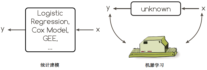
• 统计建模（statistical modeling）：统计模型是对数据分布（distribution）和数据生成过程（data-generating process）的数学描述。Kenneth Bollen认为"a model is a formal representation of a theory"。

• 机器学习（machine learning）：设计和分析一些让计算机可以自动“学习”的算法，即从数据中自动分析获得规律，并利用规律对未知数据进行预测的算法。虽然算法设计过程中也涉及统计学理论，但与统计学习相比，机器学习更关注可以实现的、行之有效的学习算法（如决策树、聚类、支持向量机、神经网络等）。

• 数据挖掘（data mining） ：从大量的数据中自动搜索隐藏于其中的知识和信息的过程，也称为数据库知识发现（Knowledge-Discovery in Databases, KDD）。数据挖掘在大数据采集和存储技术的基础上，通过统计分析、机器学习、在线分析处理、情报检索、专家系统和模式识别等诸多方法来实现具体的应用性目标。

• 小结：
  
  • 统计建模者认为世界可以用概率分布来逼近，统计建模的最终目的是获得数据的概率分布，并在此基础上进行统计推断。
  • 机器学习则不关心数据产生于什么分布，甚至认为这个世界运行的方式非常复杂、无法用概率分布来解释，因此或机器学习的目标是最小化预测误差的某种度量，它关注的是预测的精准性。
  • 从统计建模、统计学习、机器学习到数据挖掘，理论性要求下降、应用性要求上升。

2. 主成分分析（Principal Component Analysis）

2.1 思想与方法

1. 问题：

   • 当数据集包含太多的变量指标时，我们很难通过相关性分析或做成对散点图的方法来了解变量之间的关系。
   • 当数据集的样本量小于指标数 $N<K$ 时，无法对 $Y=f(X)+\varepsilon$ 进行回归分析。
   • 当我们所关心的指标（如企业发展潜力、国家治理能力等）无法直接观测时，就要在一系列可观测指标 $X$ 的基础上，构造出少数指标 $Z$ 来评判或预测 $Y$。

2. 定义：

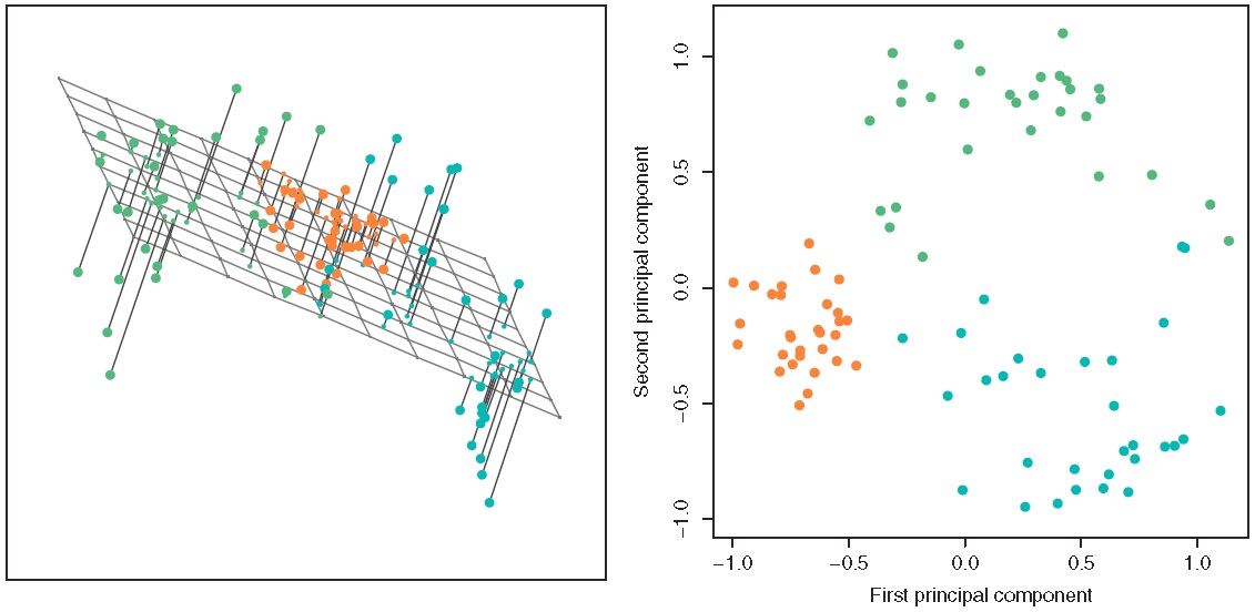
   • 主成分分析（PCA）是将多个原始变量组合为少数几个主成分，并保留绝大部分信息的降维分析技术。
   • 数学表述： 给定经过标准化处理的数据集 $X_{N \times K}$，假定存在矩阵 $\Phi _{K \times P}$所表示的超平面（其中 $P \le K$），将 $X$ 投影到 $\Phi$ 得到 $P$ 维向量：
     $$\mathop Z\limits_{N \times P} = \mathop X\limits_{N \times K} \mathop \Phi \limits_{K \times P}\\ [{z_1},{z_2},...,{z_P}] = X[{\phi _1},{\phi _2},...,{\phi _P}]$$
     若 $z_1 = X\phi_1$ 的方差满足（$\Sigma =X^TX$）：
     $$\begin{array}{l} Var\left( {{z_1}} \right) = \mathop {\max }\limits_{{\phi _1}} E\left( {\phi _1^T\Sigma {\phi _1}} \right)\\ s.t.~\phi _1^T\phi _1 = 1 \end{array}$$
     我们称 $z_1$ 为第一主成分的得分（score），$\phi_1$ 为第一主成分的载荷向量（loading），是原 $K$ 维空间中数据变异最大的方向。进而在 $\phi _2$ 与 $\phi _1$ 正交的条件下，提取第二主成分：
     $$\begin{array}{l} Var\left( {{z_2}} \right) = \mathop {\max }\limits_{{\phi _2}} E\left( {\phi _2^T\Sigma {\phi _2}} \right)\\ s.t.~\phi _2^T\phi _2 = 1\\ ~~~~~~~~\phi _1^T\phi _2 =0 \end{array}$$
     以此类推，直至得到最多 $K$ 维的向量 $Z$。
     

2.2 程序实现

library(ISLR)                            # 调用数据包
dimnames(USArrests)                      # 美国各州犯罪数据指标
apply(USArrests,2,mean)                  # 查看各指标均值和方差
apply(USArrests,2, var)

在进行主成分分析之前，需要将各指标进行标准化，否则将直接影响分析结果：

$${X_k} = \frac{{X_k^{raw} - \bar X_k^{raw}}}{{\sigma _k^{raw}}}$$

pca.out=prcomp(USArrests, scale=TRUE)    # 主成分分析，用scale=T 进行标准化，或者用x=scale(x)手动处理
pca.out                                  # 主成分载荷矩阵 Phi
names(pca.out)                           # 其他可报告的变量
head(pca.out$x)                          # 主成分得分矩阵 Z
pve=pca.out$sdev^2/sum(pca.out$sdev^2)   # 每个主成分的方差解释比
plot(pve, type="l")
cumpve=cumsum(pve)                       # 累积方差解释比
plot(cumpve, type="l")
biplot(pca.out, scale=0)                 # 前两个主成分的双标图

3. 聚类分析

3.1 什么是聚类分析？

• 定义：聚类分析（clustering）是在一个数据集中寻找子群或类的技术。
• 与主成分分析的区别：
  
  • 主成分分析通过寻找方差最大的、变量的低维组合来提取信息（$K \to P$）；
  • 聚类分析则是寻找样本的同质子类（$N \to K$）。

3.2 K均值聚类（K-means Clustering）

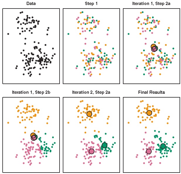
• 思想：将观测划分到事先规定数量的类中，使类内差异尽可能小。
• 公式：例如定义差异为两点之间的欧几里得距离 $\left\| \cdot \right\|$，${\left| {{C_k}} \right|}$ 为第 $k$ 类所包含的样本数。
  $$\min \sum\limits_{k = 1}^K {W\left( {{C_k}} \right)} = \frac{1}{{\left| {{C_k}} \right|}}\sum\limits_{u,v \in {C_k}} {\left\| {{x_u} - {x_v}} \right\|}$$
• 方法：
  步骤1：将每个样本随机分配一个1到K的数字，即随机设定每个样本的初始类 $k_i^0 \in \left\{ {1,2...K} \right\}$；
  步骤2：重复下列操作，直到类的分配挺直为止：
  （1）分别计算K个类的类中心 ${{\bar x}_k} = \frac{1}{{\left| {{C_k}} \right|}}\sum\limits_{i \in {C_k}} {{x_i}}$
  （2）将每个样本分配到距离其最近的类中心所在的类中，${k_i} = \mathop {\arg \min }\limits_k \sum\limits_{i \in {C_k}} {\left\| {{x_i} - {{\bar x}_k}} \right\|}$
  

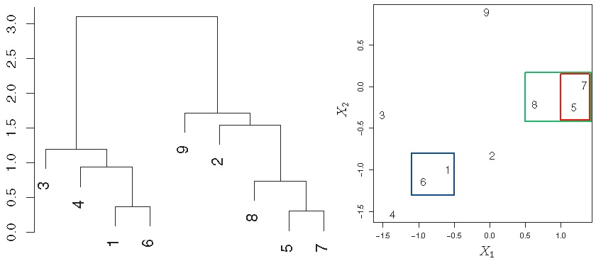
3.3 系统聚类（Hierarchical Clustering）

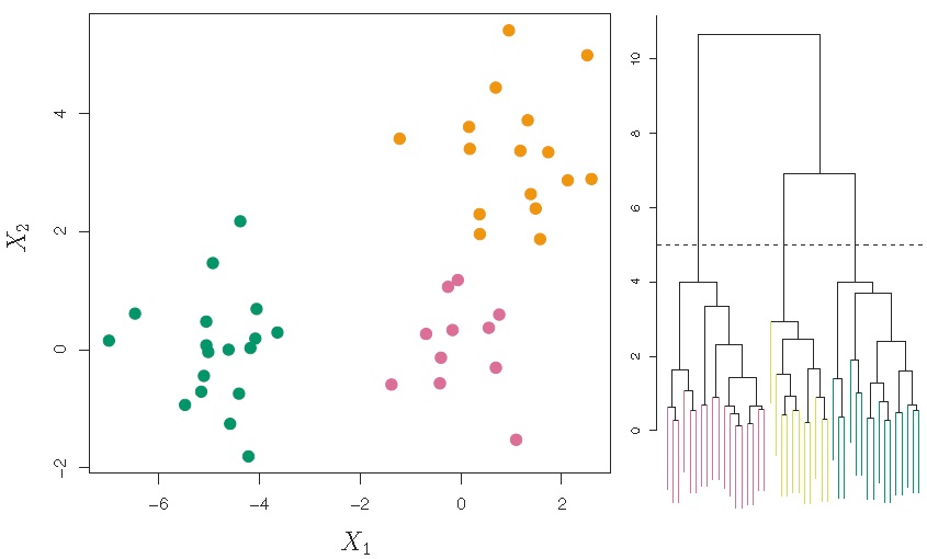
• 思想：自下而上，逐一将差异最小（距离最近）的样本合并归类。
  

• 方法：
  步骤1：将每个样本作为一个类，即设定 $N$ 个初始类，并计算两两之间的差异度（如欧氏距离）；
  步骤2：令 $i=N, N-1,...2$：
  （1）在 $i$ 个类中找到差异最小的两个类进行合并；
  （2）计算剩下的 $i-1$ 个类中两两之间的差异度。
  

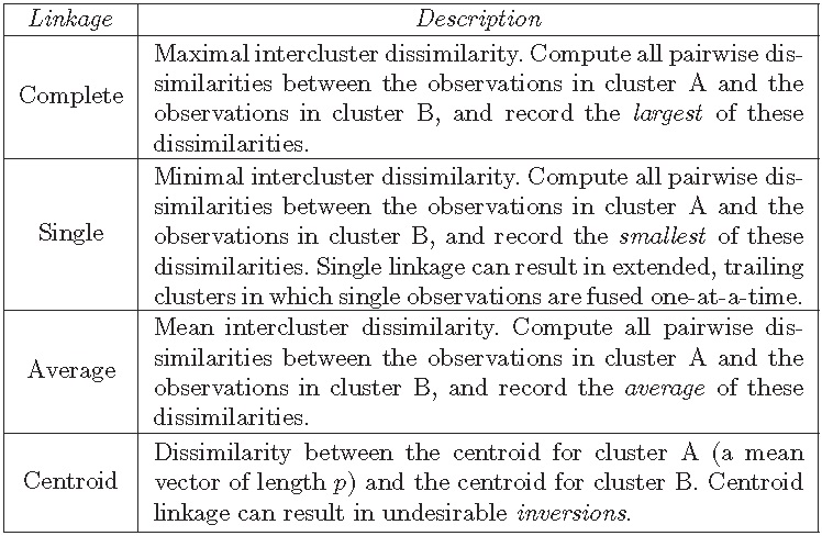
• 四种常用的类间差异度测量方法（最长距离、最短距离、类平均和重心法）：
  

3.4 程序实现

# K均值聚类
set.seed(101)
x=matrix(rnorm(100*2),100,2)           # 随机生成样本量为100、维度为2的数据集
xmean=matrix(rnorm(8,sd=4),4,2)        # 生成4组、2维的随机数
which=sample(1:4,100,replace=TRUE)     # 将100个样本随机分为4组
x=x+xmean[which,]                      # 通过改变4组数据均值的方式将其分开
plot(x,col=which,pch=19)               # 做图
km.out=kmeans(x,4,nstart=15)           # K均值聚类，K=4， 重复15次，报告最好结果
km.out
plot(x,col=km.out$cluster,cex=0.5,pch=1,lwd=2)
which=c(4,3,2,1)[which]                # 原数据分组倒序排列
km.result=data.frame(km=as.factor(km.out$cluster),which=as.factor(which), x)
table(km.result[,1:2])                 # 检查聚类结果，发现有两个样本匹配错了
km.result$miskm=(km.result$km!=km.result$which)
ggplot(km.result, aes(x=X1, y=X2, color=km, size=miskm)) +
  geom_point() +  theme_bw()
# 系统聚类
hc.complete=hclust(dist(x),method="complete") # 最长距离法 
plot(hc.complete)
hc.single=hclust(dist(x),method="single")     # 最短距离法
plot(hc.single)
hc.average=hclust(dist(x),method="average")   # 类平均法
plot(hc.average)
hc.cut=cutree(hc.complete,4)                  # 基于最长距离法的聚类结果分为4组
table(hc.cut,which)                           # 与真实数据比较，有三个样本分错
result=data.frame(x)
result$hc=as.factor(c(2,3,4,1)[hc.cut])
result$mishc=(result$hc!=which)
ggplot(result, aes(x=X1, y=X2, color=hc, size=mishc)) +
  geom_point() +  theme_bw()

4. 金融数据应用

4.1 Tsay(2013) 多支个股的主成分分析

rtn=read.table("m-5clog-9008.txt",header=T)  # 读取5支个股收益率数据
pca.cov = princomp(rtn)                      # 对协方差矩阵做主成分分析
summary(pca.cov)
pca.corr=princomp(rtn,cor=T)                 # 对相关系数矩阵做主成分分析
summary(pca.corr)
names(pca.corr)
pca2=prcomp(rtn, scale=T)                    # 用prcomp命令的结果与pca.corr一致
round(data.frame(pca.corr$sdev, pca2$sdev),3)
pca.corr$loadings
round(pca2$rotation,3)

4.2 聚类方法应用于信用卡数据

# 数据读取
credit=read.csv("Credit.csv", header=T)[,-1]
str(credit)
# 将种族等因子变量转换为数值变量
credit= credit %>%
  mutate(Gender=as.numeric(as.character(Gender)==" Male"),
         Student=as.numeric(as.character(Student)=="Yes"),
         Married=as.numeric(as.character(Married)=="Yes"),
         Ethtype=as.numeric(Ethnicity))%>%
  dplyr::select(-Ethnicity)
# 聚类分析
km.out=kmeans(credit,3,nstart=15)              
credit$km3=km.out$cluster
hc.out=hclust(dist(credit),method="complete") 
hc.cut=cutree(hc.out,3)                       
credit$hc=hc.cut
# 比较两种聚类结果 
table(hc.cut,km.out$cluster)                  
ggplot(credit, 
       aes(x=Income, y=Rating, color=as.factor(hc), shape=as.factor(km3)))+
  geom_point() +  theme_bw()

参考材料

1. L. Breiman, 2001: Statistical modeling: The two cultures, Institute of Mathematical Statistics
2. G. James, D. Vitten, T. Hastie, R. Tibshirani 著：《统计学习导论：基于R应用》，王星译，机械工业出版社，2015，（在线课程链接）
3. Ruey S. Tsay 著：《金融时间序列分析（第3版）》，王远林、王辉、潘家柱译，人民邮电出版社, 2013
   Ch09 主成分分析和因子模型.pdf5084.8kB