@zhuanxu
2017-11-30T09:46:04.000000Z
字数 7557
阅读 4840
xgboost 库使用入门
机器学习 xgboost
本文 github 地址:1-1 基本模型调用. ipynb,里面会记录自己kaggle大赛中的内容,欢迎start关注。
# 开启多行显示from IPython.core.interactiveshell import InteractiveShellInteractiveShell.ast_node_interactivity = "all"# InteractiveShell.ast_node_interactivity = "last_expr"# 显示图片%matplotlib inline%config InlineBackend.figure_format = 'retina'
数据探索
XGBoost中数据形式可以是libsvm的,libsvm作用是对稀疏特征进行优化,看个例子:
1 101:1.2 102:0.030 1:2.1 10001:300 10002:4000 2:1.2 1212:21 7777:2
每行表示一个样本,每行开头0,1表示标签,而后面的则是特征索引:数值,其他未表示都是0.
我们以判断蘑菇是否有毒为例子来做后续的训练。数据集来自:http://archive.ics.uci.edu/ml/machine-learning-databases/mushroom/ ,其中蘑菇有22个属性,将这些原始的特征加工后得到126维特征,并保存为libsvm格式,标签是表示蘑菇是否有毒。其中其中 6513 个样本做训练,1611 个样本做测试。
import xgboost as xgbfrom sklearn.metrics import accuracy_score
DMatrix is a internal data structure that used by XGBoost
which is optimized for both memory efficiency and training speed.
DMatrix 的数据来源可以是 string/numpy array/scipy.sparse/pd.DataFrame,如果是 string,则代表 libsvm 文件的路径,或者是 xgboost 可读取的二进制文件路径。
data_fold = "./data/"dtrain = xgb.DMatrix(data_fold + "agaricus.txt.train")dtest = xgb.DMatrix(data_fold + "agaricus.txt.test")
查看数据情况
(dtrain.num_col(),dtrain.num_row())(dtest.num_col(),dtest.num_row())
(127, 6513)
(127, 1611)
模型训练
基本参数设定:
- max_depth: 树的最大深度。缺省值为6,取值范围为:[1,∞]
- eta:为了防止过拟合,更新过程中用到的收缩步长。eta通过缩减特征 的权重使提升计算过程更加保守。缺省值为0.3,取值范围为:[0,1]
- silent: 0表示打印出运行时信息,取1时表示以缄默方式运行,不打印 运行时信息。缺省值为0
- objective: 定义学习任务及相应的学习目标,“binary:logistic” 表示 二分类的逻辑回归问题,输出为概率。
param = {'max_depth':2, 'eta':1, 'silent':0, 'objective':'binary:logistic' }
%time# 设置boosting迭代计算次数num_round = 2bst = xgb.train(param, dtrain, num_round)
CPU times: user 0 ns, sys: 0 ns, total: 0 ns
Wall time: 65.6 µs
此处模型输出是一个概率值,我们将其转换为0-1值,然后再计算准确率
train_preds = bst.predict(dtrain)train_predictions = [round(value) for value in train_preds]y_train = dtrain.get_label()train_accuracy = accuracy_score(y_train, train_predictions)print ("Train Accuary: %.2f%%" % (train_accuracy * 100.0))
Train Accuary: 97.77%
我们最后再测试集上看下模型的准确率的
preds = bst.predict(dtest)predictions = [round(value) for value in preds]y_test = dtest.get_label()test_accuracy = accuracy_score(y_test, predictions)print("Test Accuracy: %.2f%%" % (test_accuracy * 100.0))
Test Accuracy: 97.83%
from matplotlib import pyplotimport graphvizxgb.to_graphviz(bst, num_trees=0 )pyplot.show()

scikit-learn 接口格式
from xgboost import XGBClassifierfrom sklearn.datasets import load_svmlight_file
my_workpath = './data/'X_train,y_train = load_svmlight_file(my_workpath + 'agaricus.txt.train')X_test,y_test = load_svmlight_file(my_workpath + 'agaricus.txt.test')# 设置boosting迭代计算次数num_round = 2#bst = XGBClassifier(**params)#bst = XGBClassifier()bst =XGBClassifier(max_depth=2, learning_rate=1, n_estimators=num_round,silent=True, objective='binary:logistic')bst.fit(X_train, y_train)
XGBClassifier(base_score=0.5, booster='gbtree', colsample_bylevel=1,
       colsample_bytree=1, gamma=0, learning_rate=1, max_delta_step=0,
       max_depth=2, min_child_weight=1, missing=None, n_estimators=2,
       n_jobs=1, nthread=None, objective='binary:logistic', random_state=0,
       reg_alpha=0, reg_lambda=1, scale_pos_weight=1, seed=None,
       silent=True, subsample=1)
# 训练集上准确率train_preds = bst.predict(X_train)train_predictions = [round(value) for value in train_preds]train_accuracy = accuracy_score(y_train, train_predictions)print ("Train Accuary: %.2f%%" % (train_accuracy * 100.0))
Train Accuary: 97.77%
# 测试集上准确率# make predictionpreds = bst.predict(X_test)predictions = [round(value) for value in preds]test_accuracy = accuracy_score(y_test, predictions)print("Test Accuracy: %.2f%%" % (test_accuracy * 100.0))
Test Accuracy: 97.83%
scikit-lean 中 cv 使用
做cross_validation主要用到下面 StratifiedKFold 函数
# 设置boosting迭代计算次数num_round = 2bst =XGBClassifier(max_depth=2, learning_rate=0.1,n_estimators=num_round,silent=True, objective='binary:logistic')
from sklearn.model_selection import StratifiedKFoldfrom sklearn.model_selection import cross_val_score
kfold = StratifiedKFold(n_splits=10, random_state=7)results = cross_val_score(bst, X_train, y_train, cv=kfold)print(results)print("CV Accuracy: %.2f%% (%.2f%%)" % (results.mean()*100, results.std()*100))
[ 0.69478528  0.85276074  0.95398773  0.97235023  0.96006144  0.98771121
  1.          1.          0.96927803  0.97695853]
CV Accuracy: 93.68% (9.00%)
GridSearchcv 搜索最优解
from sklearn.model_selection import GridSearchCV
bst =XGBClassifier(max_depth=2, learning_rate=0.1, silent=True, objective='binary:logistic')
%timeparam_grid = {'n_estimators': range(1, 51, 1)}clf = GridSearchCV(bst, param_grid, "accuracy",cv=5)clf.fit(X_train, y_train)
CPU times: user 0 ns, sys: 0 ns, total: 0 ns
Wall time: 24.3 µs
clf.best_params_, clf.best_score_
({'n_estimators': 30}, 0.98418547520343924)
## 在测试集合上测试#make predictionpreds = clf.predict(X_test)predictions = [round(value) for value in preds]test_accuracy = accuracy_score(y_test, predictions)print("Test Accuracy of gridsearchcv: %.2f%%" % (test_accuracy * 100.0))
Test Accuracy of gridsearchcv: 97.27%
early-stop
我们设置验证valid集,当我们迭代过程中发现在验证集上错误率增加,则提前停止迭代。
from sklearn.model_selection import train_test_split
seed = 7test_size = 0.33X_train_part, X_validate, y_train_part, y_validate= train_test_split(X_train, y_train, test_size=test_size,random_state=seed)X_train_part.shapeX_validate.shape
(4363, 126)
(2150, 126)
# 设置boosting迭代计算次数num_round = 100bst =XGBClassifier(max_depth=2, learning_rate=0.1, n_estimators=num_round, silent=True, objective='binary:logistic')eval_set =[(X_validate, y_validate)]bst.fit(X_train_part, y_train_part, early_stopping_rounds=10, eval_metric="error",eval_set=eval_set, verbose=True)
[0] validation_0-error:0.048372
Will train until validation_0-error hasn't improved in 10 rounds.
[1] validation_0-error:0.042326
[2] validation_0-error:0.048372
[3] validation_0-error:0.042326
[4] validation_0-error:0.042326
[5] validation_0-error:0.042326
[6] validation_0-error:0.023256
[7] validation_0-error:0.042326
[8] validation_0-error:0.042326
[9] validation_0-error:0.023256
[10]    validation_0-error:0.006512
[11]    validation_0-error:0.017674
[12]    validation_0-error:0.017674
[13]    validation_0-error:0.017674
[14]    validation_0-error:0.017674
[15]    validation_0-error:0.017674
[16]    validation_0-error:0.017674
[17]    validation_0-error:0.017674
[18]    validation_0-error:0.024651
[19]    validation_0-error:0.020465
[20]    validation_0-error:0.020465
Stopping. Best iteration:
[10]    validation_0-error:0.006512
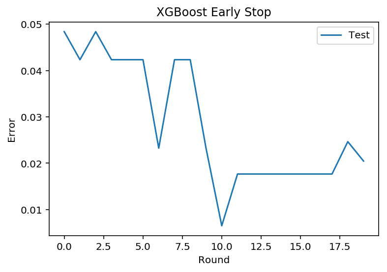
我们可以将上面的错误率进行可视化,方便我们更直观的观察
results = bst.evals_result()#print(results)epochs = len(results['validation_0']['error'])x_axis = range(0, epochs)# plot log lossfig, ax = pyplot.subplots()ax.plot(x_axis, results['validation_0']['error'], label='Test')ax.legend()pyplot.ylabel('Error')pyplot.xlabel('Round')pyplot.title('XGBoost Early Stop')pyplot.show()
# 测试集上准确率# make predictionpreds = bst.predict(X_test)predictions = [round(value) for value in preds]test_accuracy = accuracy_score(y_test, predictions)print("Test Accuracy: %.2f%%" % (test_accuracy * 100.0))
Test Accuracy: 97.27%
学习曲线
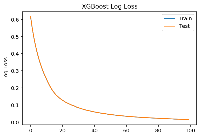
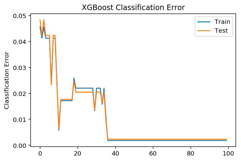
# 设置boosting迭代计算次数num_round = 100# 没有 eraly_stopbst =XGBClassifier(max_depth=2, learning_rate=0.1, n_estimators=num_round, silent=True, objective='binary:logistic')eval_set = [(X_train_part, y_train_part), (X_validate, y_validate)]bst.fit(X_train_part, y_train_part, eval_metric=["error", "logloss"], eval_set=eval_set, verbose=True)
# retrieve performance metricsresults = bst.evals_result()#print(results)epochs = len(results['validation_0']['error'])x_axis = range(0, epochs)# plot log lossfig, ax = pyplot.subplots()ax.plot(x_axis, results['validation_0']['logloss'], label='Train')ax.plot(x_axis, results['validation_1']['logloss'], label='Test')ax.legend()pyplot.ylabel('Log Loss')pyplot.title('XGBoost Log Loss')pyplot.show()# plot classification errorfig, ax = pyplot.subplots()ax.plot(x_axis, results['validation_0']['error'], label='Train')ax.plot(x_axis, results['validation_1']['error'], label='Test')ax.legend()pyplot.ylabel('Classification Error')pyplot.title('XGBoost Classification Error')pyplot.show()
# make predictionpreds = bst.predict(X_test)predictions = [round(value) for value in preds]test_accuracy = accuracy_score(y_test, predictions)print("Test Accuracy: %.2f%%" % (test_accuracy * 100.0))
Test Accuracy: 99.81%
