week02.Ng's Sequence Model Course-Homework

2018.02 Coursera

---

Operations on word vectors

Welcome to your first assignment of this week!

Because word embeddings are very computionally expensive to train, most ML practitioners will load a pre-trained set of embeddings.

After this assignment you will be able to:

• Load pre-trained word vectors, and measure similarity using cosine similarity
• Use word embeddings to solve word analogy problems such as Man is to Woman as King is to __.
• Modify word embeddings to reduce their gender bias

Let's get started! Run the following cell to load the packages you will need.

import numpy as np
from w2v_utils import *

Next, lets load the word vectors. For this assignment, we will use 50-dimensional GloVe vectors to represent words. Run the following cell to load the word_to_vec_map.

words, word_to_vec_map = read_glove_vecs('data/glove.6B.50d.txt')

You've loaded:
- words: set of words in the vocabulary.
- word_to_vec_map: dictionary mapping words to their GloVe vector representation.

You've seen that one-hot vectors do not do a good job cpaturing what words are similar. GloVe vectors provide much more useful information about the meaning of individual words. Lets now see how you can use GloVe vectors to decide how similar two words are.

1 - Cosine similarity

To measure how similar two words are, we need a way to measure the degree of similarity between two embedding vectors for the two words. Given two vectors $u$ and $v$, cosine similarity is defined as follows:

$$\text{CosineSimilarity(u, v)} = \frac {u . v} {||u||_2 ||v||_2} = cos(\theta) \tag{1}$$

where $u.v$ is the dot product (or inner product) of two vectors, $||u||_2$ is the norm (or length) of the vector $u$, and $\theta$ is the angle between $u$ and $v$. This similarity depends on the angle between $u$ and $v$. If $u$ and $v$ are very similar, their cosine similarity will be close to 1; if they are dissimilar, the cosine similarity will take a smaller value.

Figure 1: The cosine of the angle between two vectors is a measure of how similar they are

Exercise: Implement the function cosine_similarity() to evaluate similarity between word vectors.

Reminder: The norm of $u$ is defined as $||u||_2 = \sqrt{\sum_{i=1}^{n} u_i^2}$

完成代码：

# GRADED FUNCTION: cosine_similarity
def cosine_similarity(u, v):
    """
    Cosine similarity reflects the degree of similariy between u and v
    Arguments:
        u -- a word vector of shape (n,)          
        v -- a word vector of shape (n,)
    Returns:
        cosine_similarity -- the cosine similarity between u and v defined by the formula above.
    """
    distance = 0.0
    ### START CODE HERE ###
    # Compute the dot product between u and v (≈1 line)
    dot = np.matmul(np.transpose(u), v)
    # Compute the L2 norm of u (≈1 line)
    norm_u = np.linalg.norm(u, ord = 2)
    # Compute the L2 norm of v (≈1 line)
    norm_v = np.linalg.norm(v, ord = 2)
    # Compute the cosine similarity defined by formula (1) (≈1 line)
    cosine_similarity = dot / (norm_u * norm_v)
    ### END CODE HERE ###
    return cosine_similarity

测试代码

father = word_to_vec_map["father"]
mother = word_to_vec_map["mother"]
ball = word_to_vec_map["ball"]
crocodile = word_to_vec_map["crocodile"]
france = word_to_vec_map["france"]
italy = word_to_vec_map["italy"]
paris = word_to_vec_map["paris"]
rome = word_to_vec_map["rome"]
print("cosine_similarity(father, mother) = ", cosine_similarity(father, mother))
print("cosine_similarity(ball, crocodile) = ",cosine_similarity(ball, crocodile))
print("cosine_similarity(france - paris, rome - italy) = ",cosine_similarity(france - paris, rome - italy))

测试结果：

cosine_similarity(father, mother) =  0.890903844289
cosine_similarity(ball, crocodile) =  0.274392462614
cosine_similarity(france - paris, rome - italy) =  -0.675147930817

After you get the correct expected output, please feel free to modify the inputs and measure the cosine similarity between other pairs of words! Playing around the cosine similarity of other inputs will give you a better sense of how word vectors behave.

2 - Word analogy task

In the word analogy task, we complete the sentence "a is to b as c is to ____". An example is 'man is to woman as king is to queen' . In detail, we are trying to find a word d, such that the associated word vectors $e_a, e_b, e_c, e_d$ are related in the following manner: $e_b - e_a \approx e_d - e_c$. We will measure the similarity between $e_b - e_a$ and $e_d - e_c$ using cosine similarity.

Exercise: Complete the code below to be able to perform word analogies!

# GRADED FUNCTION: complete_analogy
def complete_analogy(word_a, word_b, word_c, word_to_vec_map):
    """
    Performs the word analogy task as explained above: a is to b as c is to ____. 
    Arguments:
    word_a -- a word, string
    word_b -- a word, string
    word_c -- a word, string
    word_to_vec_map -- dictionary that maps words to their corresponding vectors. 
    Returns:
    best_word --  the word such that v_b - v_a is close to v_best_word - v_c, as measured by cosine similarity
    """
    # convert words to lower case
    word_a, word_b, word_c = word_a.lower(), word_b.lower(), word_c.lower()
    ### START CODE HERE ###
    # Get the word embeddings v_a, v_b and v_c (≈1-3 lines)
    e_a, e_b, e_c = word_to_vec_map[word_a], word_to_vec_map[word_b], word_to_vec_map[word_c]
    ### END CODE HERE ###
    words = word_to_vec_map.keys()
    #words = word_to_vec_map.values()
    max_cosine_sim = -100              # Initialize max_cosine_sim to a large negative number
    best_word = None                   # Initialize best_word with None, it will help keep track of the word to output
    # loop over the whole word vector set
    for w in words:        
        # to avoid best_word being one of the input words, pass on them.
        if w in [word_a, word_b, word_c] :
            continue
        ### START CODE HERE ###
        # Compute cosine similarity between the vector (e_b - e_a) and the vector ((w's vector representation) - e_c)  (≈1 line)
        cosine_sim = cosine_similarity(e_b - e_a, word_to_vec_map[w] - e_c)
        # If the cosine_sim is more than the max_cosine_sim seen so far,
            # then: set the new max_cosine_sim to the current cosine_sim and the best_word to the current word (≈3 lines)
        if cosine_sim > max_cosine_sim:
            max_cosine_sim = cosine_sim
            best_word = w
        ### END CODE HERE ###
    return best_word

Run the cell below to test your code, this may take 1-2 minutes.

triads_to_try = [('italy', 'italian', 'spain'), ('india', 'delhi', 'japan'), ('man', 'woman', 'boy'), ('small', 'smaller', 'large')]
for triad in triads_to_try:
    print ('{} -> {} :: {} -> {}'.format( *triad, complete_analogy(*triad,word_to_vec_map)))

测试结果

italy -> italian :: spain -> spanish
india -> delhi :: japan -> tokyo
man -> woman :: boy -> girl
small -> smaller :: large -> larger

Once you get the correct expected output, please feel free to modify the input cells above to test your own analogies. Try to find some other analogy pairs that do work, but also find some where the algorithm doesn't give the right answer: For example, you can try small->smaller as big->?.

Congratulations!

You've come to the end of this assignment. Here are the main points you should remember:

• Cosine similarity a good way to compare similarity between pairs of word vectors. (Though L2 distance works too.)
• For NLP applications, using a pre-trained set of word vectors from the internet is often a good way to get started.

Even though you have finished the graded portions, we recommend you take a look too at the rest of this notebook.

Congratulations on finishing the graded portions of this notebook!

3 - Debiasing word vectors (OPTIONAL/UNGRADED)

In the following exercise, you will examine gender biases that can be reflected in a word embedding, and explore algorithms for reducing the bias. In addition to learning about the topic of debiasing, this exercise will also help hone your intuition about what word vectors are doing. This section involves a bit of linear algebra, though you can probably complete it even without being expert in linear algebra, and we encourage you to give it a shot. This portion of the notebook is optional and is not graded.

Lets first see how the GloVe word embeddings relate to gender. You will first compute a vector $g = e_{woman}-e_{man}$, where $e_{woman}$ represents the word vector corresponding to the word woman, and $e_{man}$ corresponds to the word vector corresponding to the word man. The resulting vector $g$ roughly encodes the concept of "gender". (You might get a more accurate representation if you compute $g_1 = e_{mother}-e_{father}$, $g_2 = e_{girl}-e_{boy}$, etc. and average over them. But just using $e_{woman}-e_{man}$ will give good enough results for now.)

g = word_to_vec_map['woman'] - word_to_vec_map['man']
print(g)
[-0.087144    0.2182     -0.40986    -0.03922    -0.1032      0.94165
 -0.06042     0.32988     0.46144    -0.35962     0.31102    -0.86824
  0.96006     0.01073     0.24337     0.08193    -1.02722    -0.21122
  0.695044   -0.00222     0.29106     0.5053     -0.099454    0.40445
  0.30181     0.1355     -0.0606     -0.07131    -0.19245    -0.06115
 -0.3204      0.07165    -0.13337    -0.25068714 -0.14293    -0.224957
 -0.149       0.048882    0.12191    -0.27362    -0.165476   -0.20426
  0.54376    -0.271425   -0.10245    -0.32108     0.2516     -0.33455
 -0.04371     0.01258   ]

Now, you will consider the cosine similarity of different words with gg . Consider what a positive value of similarity means vs a negative cosine similarity.

print ('List of names and their similarities with constructed vector:')
# girls and boys name
name_list = ['john', 'marie', 'sophie', 'ronaldo', 'priya', 'rahul', 'danielle', 'reza', 'katy', 'yasmin']
for w in name_list:
    print (w, cosine_similarity(word_to_vec_map[w], g))
List of names and their similarities with constructed vector:
john -0.23163356146
marie 0.315597935396
sophie 0.318687898594
ronaldo -0.312447968503
priya 0.17632041839
rahul -0.169154710392
danielle 0.243932992163
reza -0.079304296722
katy 0.283106865957
yasmin 0.233138577679

As you can see, female first names tend to have a positive cosine similarity with our constructed vector gg , while male first names tend to have a negative cosine similarity. This is not suprising, and the result seems acceptable.

But let's try with some other words.

print('Other words and their similarities:')
word_list = ['lipstick', 'guns', 'science', 'arts', 'literature', 'warrior','doctor', 'tree', 'receptionist', 
             'technology',  'fashion', 'teacher', 'engineer', 'pilot', 'computer', 'singer']
for w in word_list:
    print (w, cosine_similarity(word_to_vec_map[w], g))
Other words and their similarities:
lipstick 0.276919162564
guns -0.18884855679
science -0.0608290654093
arts 0.00818931238588
literature 0.0647250443346
warrior -0.209201646411
doctor 0.118952894109
tree -0.0708939917548
receptionist 0.330779417506
technology -0.131937324476
fashion 0.0356389462577
teacher 0.179209234318
engineer -0.0803928049452
pilot 0.00107644989919
computer -0.103303588739
singer 0.185005181365

Do you notice anything surprising? It is astonishing how these results reflect certain unhealthy gender stereotypes. For example, "computer" is closer to "man" while "literature" is closer to "woman". Ouch!

We'll see below how to reduce the bias of these vectors, using an algorithm due to Boliukbasi et al., 2016. Note that some word pairs such as "actor"/"actress" or "grandmother"/"grandfather" should remain gender specific, while other words such as "receptionist" or "technology" should be neutralized, i.e. not be gender-related. You will have to treat these two type of words differently when debiasing.

3.1 - Neutralize bias for non-gender specific words

The figure below should help you visualize what neutralizing does. If you're using a 50-dimensional word embedding, the 50 dimensional space can be split into two parts: The bias-direction $g$, and the remaining 49 dimensions, which we'll call $g_{\perp}$. In linear algebra, we say that the 49 dimensional $g_{\perp}$ is perpendicular (or "othogonal") to $g$, meaning it is at 90 degrees to $g$. The neutralization step takes a vector such as $e_{receptionist}$ and zeros out the component in the direction of $g$, giving us $e_{receptionist}^{debiased}$.

Even though $g_{\perp}$ is 49 dimensional, given the limitations of what we can draw on a screen, we illustrate it using a 1 dimensional axis below.

Figure 2: The word vector for "receptionist" represented before and after applying the neutralize operation.

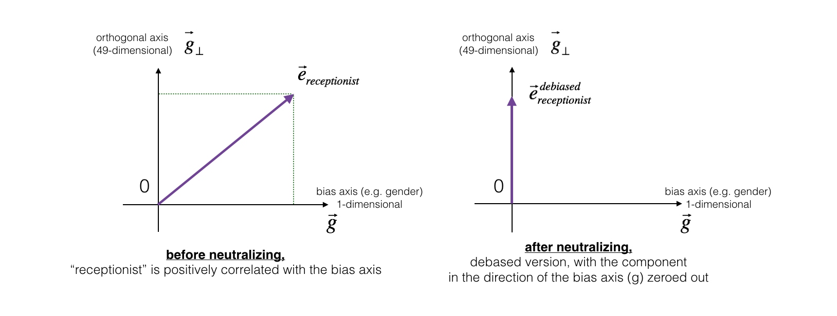
Exercise: Implement neutralize() to remove the bias of words such as "receptionist" or "scientist". Given an input embedding $e$, you can use the following formulas to compute $e^{debiased}$:

$$e^{bias\_component} = \frac{e \cdot g}{||g||_2^2} * g\tag{2}$$
$$e^{debiased} = e - e^{bias\_component}\tag{3}$$

If you are an expert in linear algebra, you may recognize $e^{bias\_component}$ as the projection of $e$ onto the direction $g$. If you're not an expert in linear algebra, don't worry about this.

def neutralize(word, g, word_to_vec_map):
    """
    Removes the bias of "word" by projecting it on the space orthogonal to the bias axis. 
    This function ensures that gender neutral words are zero in the gender subspace.
    Arguments:
        word -- string indicating the word to debias
        g -- numpy-array of shape (50,), corresponding to the bias axis (such as gender)
        word_to_vec_map -- dictionary mapping words to their corresponding vectors.
    Returns:
        e_debiased -- neutralized word vector representation of the input "word"
    """
    ### START CODE HERE ###
    # Select word vector representation of "word". Use word_to_vec_map. (≈ 1 line)
    e = word_to_vec_map[word]
    # Compute e_biascomponent using the formula give above. (≈ 1 line)
    e_biascomponent = np.matmul(e, g) / np.square( np.linalg.norm(g, ord = 2) ) * g 
    # Neutralize e by substracting e_biascomponent from it 
    # e_debiased should be equal to its orthogonal projection. (≈ 1 line)
    e_debiased = e - e_biascomponent
    ### END CODE HERE ###
    return e_debiased

e = "receptionist"
print("cosine similarity between " + e + " and g, before neutralizing: ", cosine_similarity(word_to_vec_map["receptionist"], g))
e_debiased = neutralize("receptionist", g, word_to_vec_map)
print("cosine similarity between " + e + " and g, after neutralizing: ", cosine_similarity(e_debiased, g))
cosine similarity between receptionist and g, before neutralizing:  0.330779417506
cosine similarity between receptionist and g, after neutralizing:  -3.26732746085e-17

3.2 - Equalization algorithm for gender-specific words

Next, lets see how debiasing can also be applied to word pairs such as "actress" and "actor." Equalization is applied to pairs of words that you might want to have differ only through the gender property. As a concrete example, suppose that "actress" is closer to "babysit" than "actor." By applying neutralizing to "babysit" we can reduce the gender-stereotype associated with babysitting. But this still does not guarantee that "actor" and "actress" are equidistant from "babysit." The equalization algorithm takes care of this.

The key idea behind equalization is to make sure that a particular pair of words are equi-distant from the 49-dimensional $g_\perp$. The equalization step also ensures that the two equalized steps are now the same distance from $e_{receptionist}^{debiased}$, or from any other work that has been neutralized. In pictures, this is how equalization works:

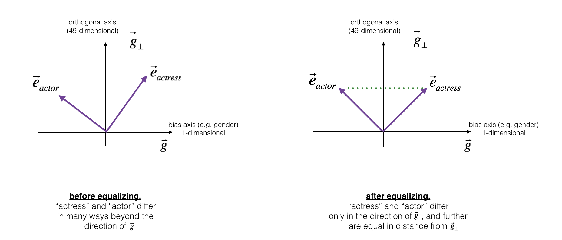
The derivation of the linear algebra to do this is a bit more complex. (See Bolukbasi et al., 2016 for details.) But the key equations are:

$$\mu = \frac{e_{w1} + e_{w2}}{2}\tag{4}$$

$$\mu_{B} = \frac {\mu \cdot \text{bias_axis}}{||\text{bias_axis}||_2^2} *\text{bias_axis} \tag{5}$$

$$\mu_{\perp} = \mu - \mu_{B} \tag{6}$$

$$e_{w1B} = \frac {e_{w1} \cdot \text{bias_axis}}{||\text{bias_axis}||_2^2} *\text{bias_axis} \tag{7}$$
$$e_{w2B} = \frac {e_{w2} \cdot \text{bias_axis}}{||\text{bias_axis}||_2^2} *\text{bias_axis} \tag{8}$$

$$e_{w1B}^{corrected} = \sqrt{ |{1 - ||\mu_{\perp} ||^2_2} |} * \frac{e_{\text{w1B}} - \mu_B} {|(e_{w1} - \mu_{\perp}) - \mu_B)|} \tag{9}$$

$$e_{w2B}^{corrected} = \sqrt{ |{1 - ||\mu_{\perp} ||^2_2} |} * \frac{e_{\text{w2B}} - \mu_B} {|(e_{w2} - \mu_{\perp}) - \mu_B)|} \tag{10}$$

$$e_1 = e_{w1B}^{corrected} + \mu_{\perp} \tag{11}$$
$$e_2 = e_{w2B}^{corrected} + \mu_{\perp} \tag{12}$$

Exercise: Implement the function below. Use the equations above to get the final equalized version of the pair of words. Good luck!

def equalize(pair, bias_axis, word_to_vec_map):
    """
    Debias gender specific words by following the equalize method described in the figure above.
    Arguments:
    pair -- pair of strings of gender specific words to debias, e.g. ("actress", "actor") 
    bias_axis -- numpy-array of shape (50,), vector corresponding to the bias axis, e.g. gender
    word_to_vec_map -- dictionary mapping words to their corresponding vectors
    Returns
    e_1 -- word vector corresponding to the first word
    e_2 -- word vector corresponding to the second word
    """
    ### START CODE HERE ###
    # Step 1: Select word vector representation of "word". Use word_to_vec_map. (≈ 2 lines)
    w1, w2 = pair
    e_w1, e_w2 = word_to_vec_map[w1], word_to_vec_map[w2]
    # Step 2: Compute the mean of e_w1 and e_w2 (≈ 1 line)
    mu = (e_w1 + e_w2) / 2
    # Step 3: Compute the projections of mu over the bias axis and the orthogonal axis (≈ 2 lines)
    mu_B = np.matmul(mu, bias_axis) / np.square(np.linalg.norm(bias_axis, ord = 2)) * bias_axis
    mu_orth = mu - mu_B
    # Step 4: Use equations (7) and (8) to compute e_w1B and e_w2B (≈2 lines)
    e_w1B = np.matmul(e_w1, bias_axis) / np.square(np.linalg.norm(bias_axis, ord = 2)) * bias_axis
    e_w2B = np.matmul(e_w1, bias_axis) / np.square(np.linalg.norm(bias_axis, ord = 2)) * bias_axis
    # Step 5: Adjust the Bias part of e_w1B and e_w2B using the formulas (9) and (10) given above (≈2 lines)
    corrected_e_w1B = np.sqrt( np.fabs( 1 - np.linalg.norm(mu_orth) ) ) * (e_w1B - mu_B) / np.fabs( (e_w1 - mu_orth) - mu_B )
    corrected_e_w2B = np.sqrt( np.fabs( 1 - np.linalg.norm(mu_orth) ) ) * (e_w2B - mu_B) / np.fabs( (e_w2 - mu_orth) - mu_B )
    # Step 6: Debias by equalizing e1 and e2 to the sum of their corrected projections (≈2 lines)
    e1 = corrected_e_w1B + mu_orth
    e2 = corrected_e_w2B + mu_orth
    ### END CODE HERE ###
    return e1, e2

print("cosine similarities before equalizing:")
print("cosine_similarity(word_to_vec_map[\"man\"], gender) = ", cosine_similarity(word_to_vec_map["man"], g))
print("cosine_similarity(word_to_vec_map[\"woman\"], gender) = ", cosine_similarity(word_to_vec_map["woman"], g))
print()
e1, e2 = equalize(("man", "woman"), g, word_to_vec_map)
print("cosine similarities after equalizing:")
print("cosine_similarity(e1, gender) = ", cosine_similarity(e1, g))
print("cosine_similarity(e2, gender) = ", cosine_similarity(e2, g))

cosine similarities before equalizing:
cosine_similarity(word_to_vec_map["man"], gender) =  -0.117110957653
cosine_similarity(word_to_vec_map["woman"], gender) =  0.356666188463
cosine similarities after equalizing:
cosine_similarity(e1, gender) =  -0.668634505208
cosine_similarity(e2, gender) =  -0.668634505208

Expected Output:

cosine similarities before equalizing:

cosine_similarity(word_to_vec_map["man"], gender) = -0.117110957653
cosine_similarity(word_to_vec_map["woman"], gender) =   0.356666188463

cosine similarities after equalizing:

cosine_similarity(u1, gender) = -0.700436428931
cosine_similarity(u2, gender) = 0.700436428931

Please feel free to play with the input words in the cell above, to apply equalization to other pairs of words.

These debiasing algorithms are very helpful for reducing bias, but are not perfect and do not eliminate all traces of bias. For example, one weakness of this implementation was that the bias direction $g$ was defined using only the pair of words woman and man. As discussed earlier, if $g$ were defined by computing $g_1 = e_{woman} - e_{man}$; $g_2 = e_{mother} - e_{father}$; $g_3 = e_{girl} - e_{boy}$; and so on and averaging over them, you would obtain a better estimate of the "gender" dimension in the 50 dimensional word embedding space. Feel free to play with such variants as well.

Congratulations

You have come to the end of this notebook, and have seen a lot of the ways that word vectors can be used as well as modified.

Congratulations on finishing this notebook!

References:
- The debiasing algorithm is from Bolukbasi et al., 2016, Man is to Computer Programmer as Woman is to Homemaker? Debiasing Word Embeddings
- The GloVe word embeddings were due to Jeffrey Pennington, Richard Socher, and Christopher D. Manning. (https://nlp.stanford.edu/projects/glove/)

Emojify!

Welcome to the second assignment of Week 2. You are going to use word vector representations to build an Emojifier.

Have you ever wanted to make your text messages more expressive? Your emojifier app will help you do that. So rather than writing "Congratulations on the promotion! Lets get coffee and talk. Love you!" the emojifier can automatically turn this into "Congratulations on the promotion! 👍 Lets get coffee and talk. ☕️ Love you! ❤️"

You will implement a model which inputs a sentence (such as "Let's go see the baseball game tonight!") and finds the most appropriate emoji to be used with this sentence (⚾️). In many emoji interfaces, you need to remember that ❤️ is the "heart" symbol rather than the "love" symbol. But using word vectors, you'll see that even if your training set explicitly relates only a few words to a particular emoji, your algorithm will be able to generalize and associate words in the test set to the same emoji even if those words don't even appear in the training set. This allows you to build an accurate classifier mapping from sentences to emojis, even using a small training set.

In this exercise, you'll start with a baseline model (Emojifier-V1) using word embeddings, then build a more sophisticated model (Emojifier-V2) that further incorporates an LSTM.

Lets get started! Run the following cell to load the package you are going to use.

import numpy as np
from emo_utils import *
import emoji
import matplotlib.pyplot as plt
%matplotlib inline

1 - Baseline model: Emojifier-V1

1.1 - Dataset EMOJISET

Let's start by building a simple baseline classifier.

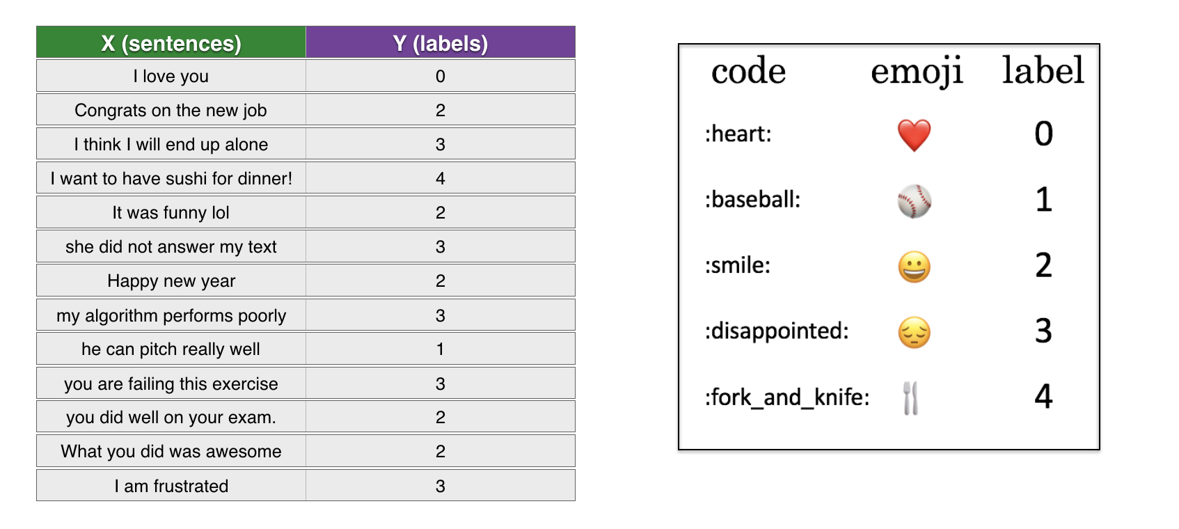
You have a tiny dataset (X, Y) where:
- X contains 127 sentences (strings)
- Y contains a integer label between 0 and 4 corresponding to an emoji for each sentence

Figure 1: EMOJISET - a classification problem with 5 classes. A few examples of sentences are given here.

Let's load the dataset using the code below. We split the dataset between training (127 examples) and testing (56 examples).

X_train, Y_train = read_csv('data/train_emoji.csv')
X_test, Y_test = read_csv('data/tesss.csv')

maxLen = len(max(X_train, key=len).split())

Run the following cell to print sentences from X_train and corresponding labels from Y_train. Change index to see different examples. Because of the font the iPython notebook uses, the heart emoji may be colored black rather than red.

index = 1
print(X_train[index], label_to_emoji(Y_train[index]))

1.2 - Overview of the Emojifier-V1

In this part, you are going to implement a baseline model called "Emojifier-v1".

Figure 2: Baseline model (Emojifier-V1).

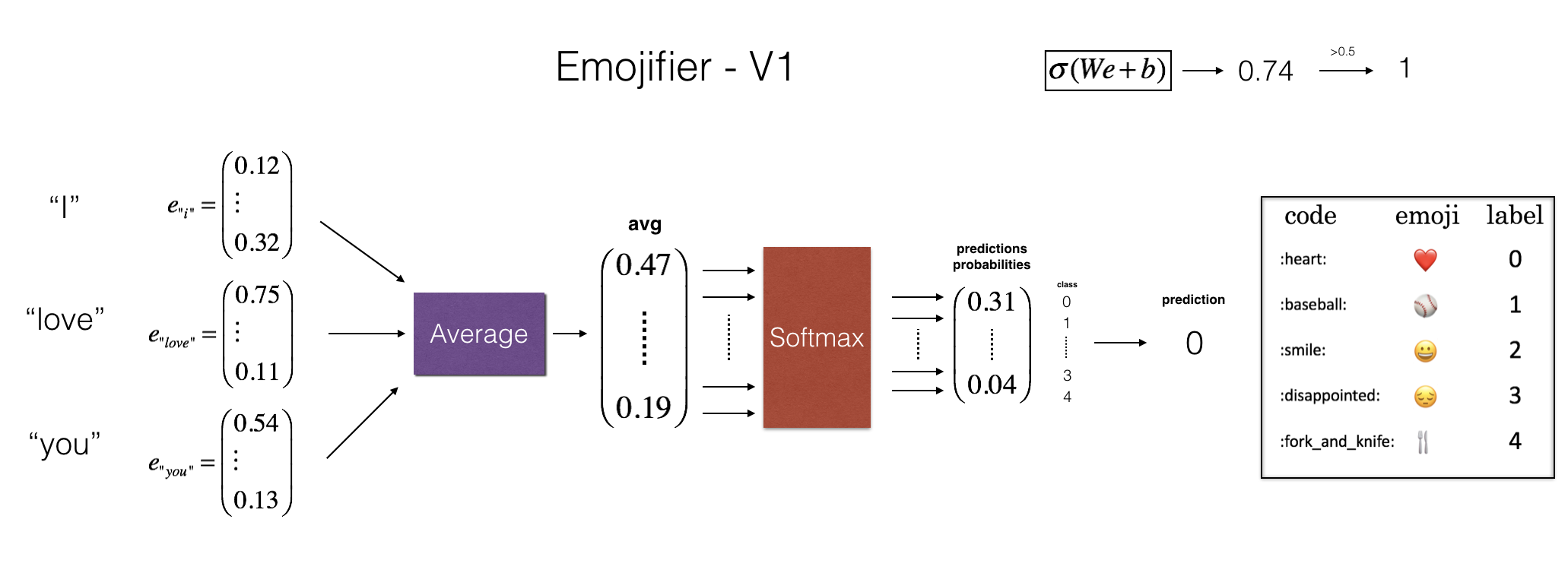
The input of the model is a string corresponding to a sentence (e.g. "I love you). In the code, the output will be a probability vector of shape (1,5), that you then pass in an argmax layer to extract the index of the most likely emoji output.

To get our labels into a format suitable for training a softmax classifier, lets convert $Y$ from its current shape current shape $(m, 1)$ into a "one-hot representation" $(m, 5)$, where each row is a one-hot vector giving the label of one example, You can do so using this next code snipper. Here, Y_oh stands for "Y-one-hot" in the variable names Y_oh_train and Y_oh_test:

Y_oh_train = convert_to_one_hot(Y_train, C = 5)
Y_oh_test = convert_to_one_hot(Y_test, C = 5)

Let's see what convert_to_one_hot() did. Feel free to change index to print out different values.

index = 50
print(Y_train[index], "is converted into one hot", Y_oh_train[index])

All the data is now ready to be fed into the Emojify-V1 model. Let's implement the model!

1.3 - Implementing Emojifier-V1

As shown in Figure (2), the first step is to convert an input sentence into the word vector representation, which then get averaged together. Similar to the previous exercise, we will use pretrained 50-dimensional GloVe embeddings. Run the following cell to load the word_to_vec_map, which contains all the vector representations.

word_to_index, index_to_word, word_to_vec_map = read_glove_vecs('data/glove.6B.50d.txt')

You've loaded:
- word_to_index: dictionary mapping from words to their indices in the vocabulary (400,001 words, with the valid indices ranging from 0 to 400,000)
- index_to_word: dictionary mapping from indices to their corresponding words in the vocabulary
- word_to_vec_map: dictionary mapping words to their GloVe vector representation.

Run the following cell to check if it works.

word = "cucumber"
index = 289846
print("the index of", word, "in the vocabulary is", word_to_index[word])
print("the", str(index) + "th word in the vocabulary is", index_to_word[index])

Exercise: Implement sentence_to_avg(). You will need to carry out two steps:
1. Convert every sentence to lower-case, then split the sentence into a list of words. X.lower() and X.split() might be useful.
2. For each word in the sentence, access its GloVe representation. Then, average all these values.

# GRADED FUNCTION: sentence_to_avg
def sentence_to_avg(sentence, word_to_vec_map):
    """
    Converts a sentence (string) into a list of words (strings). Extracts the GloVe representation of each word
    and averages its value into a single vector encoding the meaning of the sentence.
    Arguments:
    sentence -- string, one training example from X
    word_to_vec_map -- dictionary mapping every word in a vocabulary into its 50-dimensional vector representation
    Returns:
    avg -- average vector encoding information about the sentence, numpy-array of shape (50,)
    """
    ### START CODE HERE ###
    # Step 1: Split sentence into list of lower case words (≈ 1 line)
    words = sentence.lower().split()
    # Initialize the average word vector, should have the same shape as your word vectors.
    avg = np.zeros( (50, ) )
    # Step 2: average the word vectors. You can loop over the words in the list "words".
    for w in words:
        avg += word_to_vec_map[w]
    avg = avg / len(words)
    ### END CODE HERE ###
    return avg

avg = sentence_to_avg("Morrocan couscous is my favorite dish", word_to_vec_map)
print("avg = ", avg)

avg =  [-0.008005    0.56370833 -0.50427333  0.258865    0.55131103  0.03104983
 -0.21013718  0.16893933 -0.09590267  0.141784   -0.15708967  0.18525867
  0.6495785   0.38371117  0.21102167  0.11301667  0.02613967  0.26037767
  0.05820667 -0.01578167 -0.12078833 -0.02471267  0.4128455   0.5152061
  0.38756167 -0.898661   -0.535145    0.33501167  0.68806933 -0.2156265
  1.797155    0.10476933 -0.36775333  0.750785    0.10282583  0.348925
 -0.27262833  0.66768    -0.10706167 -0.283635    0.59580117  0.28747333
 -0.3366635   0.23393817  0.34349183  0.178405    0.1166155  -0.076433
  0.1445417   0.09808667]

Model

You now have all the pieces to finish implementing the model() function. After using sentence_to_avg() you need to pass the average through forward propagation, compute the cost, and then backpropagate to update the softmax's parameters.

Exercise: Implement the model() function described in Figure (2). Assuming here that $Yoh$ ("Y one hot") is the one-hot encoding of the output labels, the equations you need to implement in the forward pass and to compute the cross-entropy cost are:

$$z^{(i)} = W . avg^{(i)} + b$$
$$a^{(i)} = softmax(z^{(i)})$$
$$\mathcal{L}^{(i)} = - \sum_{k = 0}^{n_y - 1} Yoh^{(i)}_k * log(a^{(i)}_k)$$

It is possible to come up with a more efficient vectorized implementation. But since we are using a for-loop to convert the sentences one at a time into the avg^{(i)} representation anyway, let's not bother this time.

We provided you a function softmax().

# GRADED FUNCTION: model
def model(X, Y, word_to_vec_map, learning_rate = 0.01, num_iterations = 400):
    """
    Model to train word vector representations in numpy.
    Arguments:
    X -- input data, numpy array of sentences as strings, of shape (m, 1)
    Y -- labels, numpy array of integers between 0 and 7, numpy-array of shape (m, 1)
    word_to_vec_map -- dictionary mapping every word in a vocabulary into its 50-dimensional vector representation
    learning_rate -- learning_rate for the stochastic gradient descent algorithm
    num_iterations -- number of iterations
    Returns:
    pred -- vector of predictions, numpy-array of shape (m, 1)
    W -- weight matrix of the softmax layer, of shape (n_y, n_h)
    b -- bias of the softmax layer, of shape (n_y,)
    """
    np.random.seed(1)
    # Define number of training examples
    m = Y.shape[0]                          # number of training examples
    n_y = 5                                 # number of classes  
    n_h = 50                                # dimensions of the GloVe vectors 
    # Initialize parameters using Xavier initialization
    W = np.random.randn(n_y, n_h) / np.sqrt(n_h)
    b = np.zeros((n_y,))
    # Convert Y to Y_onehot with n_y classes
    Y_oh = convert_to_one_hot(Y, C = n_y) 
    # Optimization loop
    for t in range(num_iterations):                       # Loop over the number of iterations
        for i in range(m):                                # Loop over the training examples
            ### START CODE HERE ### (≈ 4 lines of code)
            # Average the word vectors of the words from the i'th training example
            avg = sentence_to_avg(X[i], word_to_vec_map)
            # Forward propagate the avg through the softmax layer
            z = np.matmul(W, avg) + b
            a = softmax(z)
            # Compute cost using the i'th training label's one hot representation and "A" (the output of the softmax)
            cost = - np.sum( Y_oh[i, :] * np.log( a ) )
            ### END CODE HERE ###
            # Compute gradients 
            dz = a - Y_oh[i]
            dW = np.dot(dz.reshape(n_y,1), avg.reshape(1, n_h))
            db = dz
            # Update parameters with Stochastic Gradient Descent
            W = W - learning_rate * dW
            b = b - learning_rate * db
        if t % 100 == 0:
            print("Epoch: " + str(t) + " --- cost = " + str(cost))
            pred = predict(X, Y, W, b, word_to_vec_map)
    return pred, W, b

print(X_train.shape)
print(Y_train.shape)
print(np.eye(5)[Y_train.reshape(-1)].shape)
print(X_train[0])
print(type(X_train))
Y = np.asarray([5,0,0,5, 4, 4, 4, 6, 6, 4, 1, 1, 5, 6, 6, 3, 6, 3, 4, 4])
print(Y.shape)
X = np.asarray(['I am going to the bar tonight', 'I love you', 'miss you my dear',
 'Lets go party and drinks','Congrats on the new job','Congratulations',
 'I am so happy for you', 'Why are you feeling bad', 'What is wrong with you',
 'You totally deserve this prize', 'Let us go play football',
 'Are you down for football this afternoon', 'Work hard play harder',
 'It is suprising how people can be dumb sometimes',
 'I am very disappointed','It is the best day in my life',
 'I think I will end up alone','My life is so boring','Good job',
 'Great so awesome'])
print(X.shape)
print(np.eye(5)[Y_train.reshape(-1)].shape)
print(type(X_train))

(132,)
(132,)
(132, 5)
never talk to me again
<class 'numpy.ndarray'>
(20,)
(20,)
(132, 5)
<class 'numpy.ndarray'>

Run the next cell to train your model and learn the softmax parameters (W,b).

pred, W, b = model(X_train, Y_train, word_to_vec_map)
print(pred)

Epoch: 0 --- cost = 1.95204988128
Accuracy: 0.348484848485
Epoch: 100 --- cost = 0.0797181872601
Accuracy: 0.931818181818
Epoch: 200 --- cost = 0.0445636924368
Accuracy: 0.954545454545
Epoch: 300 --- cost = 0.0343226737879
Accuracy: 0.969696969697

1.4 - Examining test set performance

print("Training set:")
pred_train = predict(X_train, Y_train, W, b, word_to_vec_map)
print('Test set:')
pred_test = predict(X_test, Y_test, W, b, word_to_vec_map)

Training set:
Accuracy: 0.977272727273
Test set:
Accuracy: 0.857142857143

Random guessing would have had 20% accuracy given that there are 5 classes. This is pretty good performance after training on only 127 examples.

In the training set, the algorithm saw the sentence "I love you" with the label ❤️. You can check however that the word "adore" does not appear in the training set. Nonetheless, lets see what happens if you write "I adore you."

X_my_sentences = np.array(["i adore you", "i love you", "funny lol", "lets play with a ball", "food is ready", "not feeling happy"])
Y_my_labels = np.array([[0], [0], [2], [1], [4],[3]])
pred = predict(X_my_sentences, Y_my_labels , W, b, word_to_vec_map)
print_predictions(X_my_sentences, pred)

Accuracy: 0.833333333333
i adore you ❤️
i love you ❤️
funny lol 😄
lets play with a ball ⚾
food is ready 🍴
not feeling happy 😄

Amazing! Because adore has a similar embedding as love, the algorithm has generalized correctly even to a word it has never seen before. Words such as heart, dear, beloved or adore have embedding vectors similar to love, and so might work too---feel free to modify the inputs above and try out a variety of input sentences. How well does it work?

Note though that it doesn't get "not feeling happy" correct. This algorithm ignores word ordering, so is not good at understanding phrases like "not happy."

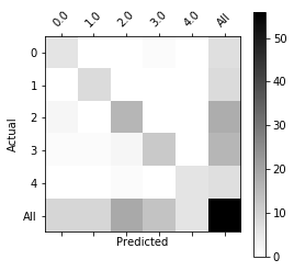
Printing the confusion matrix can also help understand which classes are more difficult for your model. A confusion matrix shows how often an example whose label is one class ("actual" class) is mislabeled by the algorithm with a different class ("predicted" class).

print(Y_test.shape)
print('           '+ label_to_emoji(0)+ '    ' + label_to_emoji(1) + '    ' +  label_to_emoji(2)+ '    ' + label_to_emoji(3)+'   ' + label_to_emoji(4))
print(pd.crosstab(Y_test, pred_test.reshape(56,), rownames=['Actual'], colnames=['Predicted'], margins=True))
plot_confusion_matrix(Y_test, pred_test)

(56,)
           ❤️    ⚾    😄    😞   🍴
Predicted  0.0  1.0  2.0  3.0  4.0  All
Actual                                 
0            6    0    0    1    0    7
1            0    8    0    0    0    8
2            2    0   16    0    0   18
3            1    1    2   12    0   16
4            0    0    1    0    6    7
All          9    9   19   13    6   56

What you should remember from this part:
- Even with a 127 training examples, you can get a reasonably good model for Emojifying. This is due to the generalization power word vectors gives you.
- Emojify-V1 will perform poorly on sentences such as "This movie is not good and not enjoyable" because it doesn't understand combinations of words--it just averages all the words' embedding vectors together, without paying attention to the ordering of words. You will build a better algorithm in the next part.

2 - Emojifier-V2: Using LSTMs in Keras:

Let's build an LSTM model that takes as input word sequences. This model will be able to take word ordering into account. Emojifier-V2 will continue to use pre-trained word embeddings to represent words, but will feed them into an LSTM, whose job it is to predict the most appropriate emoji.

Run the following cell to load the Keras packages.

import numpy as np
np.random.seed(0)
from keras.models import Model
from keras.layers import Dense, Input, Dropout, LSTM, Activation
from keras.layers.embeddings import Embedding
from keras.preprocessing import sequence
from keras.initializers import glorot_uniform
np.random.seed(1)

2.1 - Overview of the model

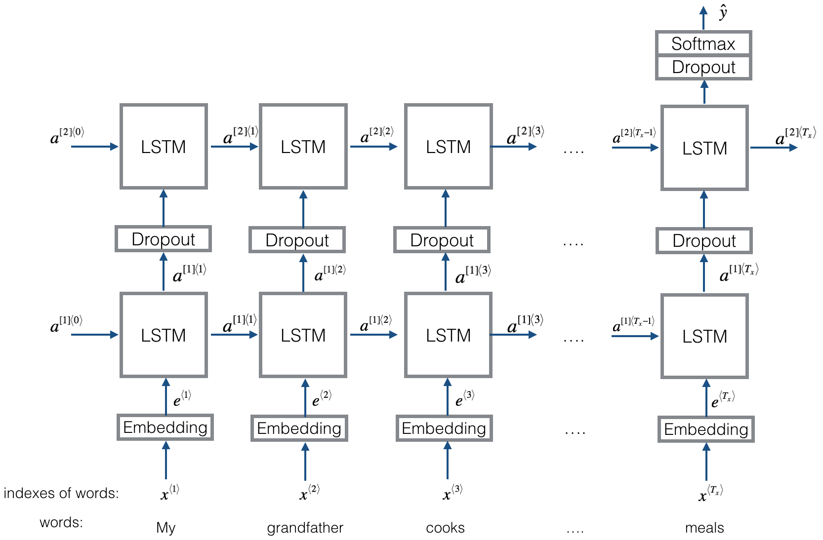
Here is the Emojifier-v2 you will implement:

Figure 3: Emojifier-V2. A 2-layer LSTM sequence classifier.

2.2 Keras and mini-batching

In this exercise, we want to train Keras using mini-batches. However, most deep learning frameworks require that all sequences in the same mini-batch have the same length. This is what allows vectorization to work: If you had a 3-word sentence and a 4-word sentence, then the computations needed for them are different (one takes 3 steps of an LSTM, one takes 4 steps) so it's just not possible to do them both at the same time.

The common solution to this is to use padding. Specifically, set a maximum sequence length, and pad all sequences to the same length. For example, of the maximum sequence length is 20, we could pad every sentence with "0"s so that each input sentence is of length 20. Thus, a sentence "i love you" would be represented as $(e_{i}, e_{love}, e_{you}, \vec{0}, \vec{0}, \ldots, \vec{0})$. In this example, any sentences longer than 20 words would have to be truncated. One simple way to choose the maximum sequence length is to just pick the length of the longest sentence in the training set.

2.3 - The Embedding layer

In Keras, the embedding matrix is represented as a "layer", and maps positive integers (indices corresponding to words) into dense vectors of fixed size (the embedding vectors). It can be trained or initialized with a pretrained embedding. In this part, you will learn how to create an Embedding() layer in Keras, initialize it with the GloVe 50-dimensional vectors loaded earlier in the notebook. Because our training set is quite small, we will not update the word embeddings but will instead leave their values fixed. But in the code below, we'll show you how Keras allows you to either train or leave fixed this layer.

The Embedding() layer takes an integer matrix of size (batch size, max input length) as input. This corresponds to sentences converted into lists of indices (integers), as shown in the figure below.

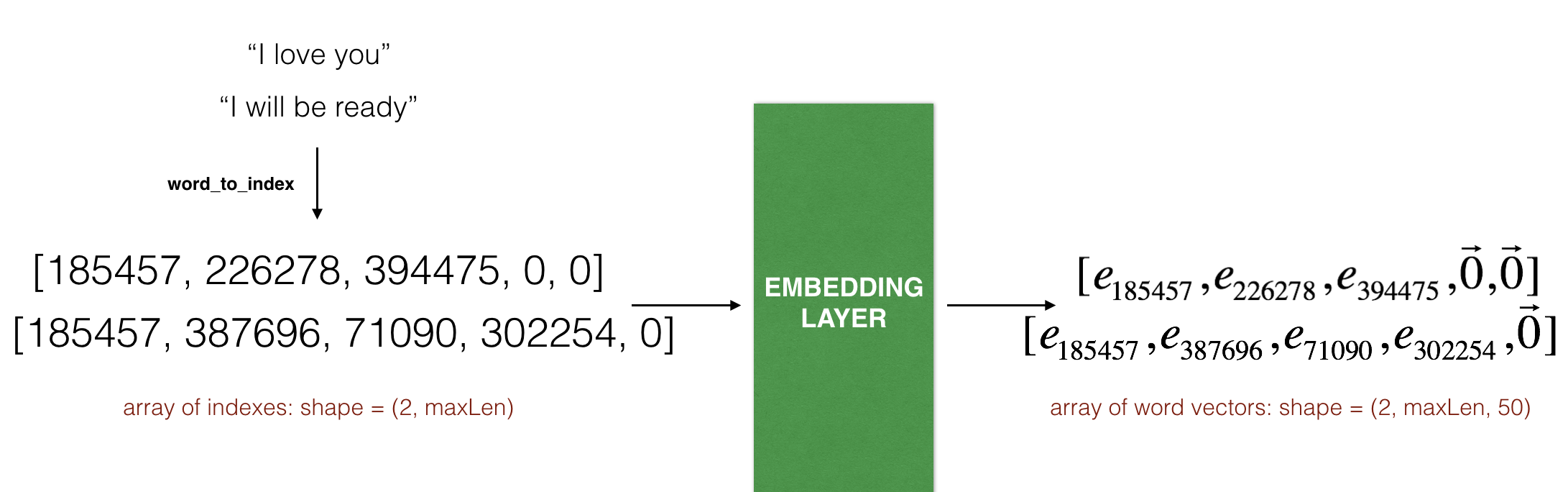
Figure 4: Embedding layer. This example shows the propagation of two examples through the embedding layer. Both have been zero-padded to a length of max_len=5. The final dimension of the representation is (2,max_len,50) because the word embeddings we are using are 50 dimensional.

The largest integer (i.e. word index) in the input should be no larger than the vocabulary size. The layer outputs an array of shape (batch size, max input length, dimension of word vectors).

The first step is to convert all your training sentences into lists of indices, and then zero-pad all these lists so that their length is the length of the longest sentence.

Exercise: Implement the function below to convert X (array of sentences as strings) into an array of indices corresponding to words in the sentences. The output shape should be such that it can be given to Embedding() (described in Figure 4).

# GRADED FUNCTION: sentences_to_indices
def sentences_to_indices(X, word_to_index, max_len):
    """
    Converts an array of sentences (strings) into an array of indices corresponding to words in the sentences.
    The output shape should be such that it can be given to `Embedding()` (described in Figure 4). 
    Arguments:
    X -- array of sentences (strings), of shape (m, 1)
    word_to_index -- a dictionary containing the each word mapped to its index
    max_len -- maximum number of words in a sentence. You can assume every sentence in X is no longer than this. 
    Returns:
    X_indices -- array of indices corresponding to words in the sentences from X, of shape (m, max_len)
    """
    m = X.shape[0]                                   # number of training examples
    ### START CODE HERE ###
    # Initialize X_indices as a numpy matrix of zeros and the correct shape (≈ 1 line)
    X_indices = np.zeros((m, max_len))
    for i in range(m):                               # loop over training examples
        # Convert the ith training sentence in lower case and split is into words. You should get a list of words.
        sentence_words = X[i].lower().split( )
        # Initialize j to 0
        j = 0
        # Loop over the words of sentence_words
        for w in sentence_words:
            # Set the (i,j)th entry of X_indices to the index of the correct word.
            X_indices[i, j] = word_to_index[w]
            # Increment j to j + 1
            j = j + 1
    ### END CODE HERE ###
    return X_indices

Run the following cell to check what sentences_to_indices() does, and check your results.

X1 = np.array(["funny lol", "lets play baseball", "food is ready for you"])
X1_indices = sentences_to_indices(X1,word_to_index, max_len = 5)
print("X1 =", X1)
print("X1_indices =", X1_indices)
X1 = ['funny lol' 'lets play baseball' 'food is ready for you']
X1_indices = [[ 155345.  225122.       0.       0.       0.]
 [ 220930.  286375.   69714.       0.       0.]
 [ 151204.  192973.  302254.  151349.  394475.]]

Let's build the Embedding() layer in Keras, using pre-trained word vectors. After this layer is built, you will pass the output of sentences_to_indices() to it as an input, and the Embedding() layer will return the word embeddings for a sentence.

Exercise: Implement pretrained_embedding_layer(). You will need to carry out the following steps:
1. Initialize the embedding matrix as a numpy array of zeroes with the correct shape.
2. Fill in the embedding matrix with all the word embeddings extracted from word_to_vec_map.
3. Define Keras embedding layer. Use Embedding(). Be sure to make this layer non-trainable, by setting trainable = False when calling Embedding(). If you were to set trainable = True, then it will allow the optimization algorithm to modify the values of the word embeddings.
4. Set the embedding weights to be equal to the embedding matrix

# GRADED FUNCTION: pretrained_embedding_layer
def pretrained_embedding_layer(word_to_vec_map, word_to_index):
    """
    Creates a Keras Embedding() layer and loads in pre-trained GloVe 50-dimensional vectors.
    Arguments:
    word_to_vec_map -- dictionary mapping words to their GloVe vector representation.
    word_to_index -- dictionary mapping from words to their indices in the vocabulary (400,001 words)
    Returns:
    embedding_layer -- pretrained layer Keras instance
    """
    vocab_len = len(word_to_index) + 1                  # adding 1 to fit Keras embedding (requirement)
    emb_dim = word_to_vec_map["cucumber"].shape[0]      # define dimensionality of your GloVe word vectors (= 50)
    ### START CODE HERE ###
    # Initialize the embedding matrix as a numpy array of zeros of shape (vocab_len, dimensions of word vectors = emb_dim)
    emb_matrix = np.zeros((vocab_len, emb_dim))
    # Set each row "index" of the embedding matrix to be the word vector representation of the "index"th word of the vocabulary
    for word, index in word_to_index.items():
        emb_matrix[index, :] = word_to_vec_map[word]
    # Define Keras embedding layer with the correct output/input sizes, make it trainable. Use Embedding(...). Make sure to set trainable=False. 
    embedding_layer = Embedding(input_dim = vocab_len, output_dim = emb_dim, trainable = False )
    ### END CODE HERE ###
    # Build the embedding layer, it is required before setting the weights of the embedding layer. Do not modify the "None".
    embedding_layer.build((None,))
    # Set the weights of the embedding layer to the embedding matrix. Your layer is now pretrained.
    embedding_layer.set_weights([emb_matrix])
    return embedding_layer

embedding_layer = pretrained_embedding_layer(word_to_vec_map, word_to_index)
print("weights[0][8][3] =", embedding_layer.get_weights()[0][9][3])
weights[0][10][3] = -0.3403

2.3 Building the Emojifier-V2

Lets now build the Emojifier-V2 model. You will do so using the embedding layer you have built, and feed its output to an LSTM network.

Figure 3: Emojifier-v2. A 2-layer LSTM sequence classifier.

Exercise: Implement Emojify_V2(), which builds a Keras graph of the architecture shown in Figure 3. The model takes as input an array of sentences of shape (m, max_len, ) defined by input_shape. It should output a softmax probability vector of shape (m, C = 5). You may need Input(shape = ..., dtype = '...'), LSTM(), Dropout(), Dense(), and Activation().

# GRADED FUNCTION: Emojify_V2
def Emojify_V2(input_shape, word_to_vec_map, word_to_index):
    """
    Function creating the Emojify-v2 model's graph.
    Arguments:
    input_shape -- shape of the input, usually (max_len,)
    word_to_vec_map -- dictionary mapping every word in a vocabulary into its 50-dimensional vector representation
    word_to_index -- dictionary mapping from words to their indices in the vocabulary (400,001 words)
    Returns:
    model -- a model instance in Keras
    """
    ### START CODE HERE ###
    # Define sentence_indices as the input of the graph, it should be of shape input_shape and dtype 'int32' (as it contains indices).
    sentence_indices = Input(shape = input_shape, dtype = 'int32')
    # Create the embedding layer pretrained with GloVe Vectors (≈1 line)
    embedding_layer = pretrained_embedding_layer(word_to_vec_map, word_to_index)
    # Propagate sentence_indices through your embedding layer, you get back the embeddings
    embeddings = embedding_layer(sentence_indices)   
    # Propagate the embeddings through an LSTM layer with 128-dimensional hidden state
    # Be careful, the returned output should be a batch of sequences.
    X = LSTM(units = 128,  activation='tanh', return_sequences =True)(embeddings)
    # Add dropout with a probability of 0.5
    X = Dropout(rate = 0.5)(X)
    # Propagate X trough another LSTM layer with 128-dimensional hidden state
    # Be careful, the returned output should be a single hidden state, not a batch of sequences.
    X = LSTM(units = 128,  activation='tanh')(X)
    # Add dropout with a probability of 0.5
    X = Dropout(rate = 0.5)(X)
    # Propagate X through a Dense layer with softmax activation to get back a batch of 5-dimensional vectors.
    X = Dense(5, activation='softmax')(X)
    # Add a softmax activation
    X = Activation('softmax')(X)
    # Create Model instance which converts sentence_indices into X.
    model = Model(inputs = [sentence_indices], outputs = [X])
    ### END CODE HERE ###
    return model

Run the following cell to create your model and check its summary. Because all sentences in the dataset are less than 10 words, we chose max_len = 10. You should see your architecture, it uses "20,223,927" parameters, of which 20,000,050 (the word embeddings) are non-trainable, and the remaining 223,877 are. Because our vocabulary size has 400,001 words (with valid indices from 0 to 400,000) there are 400,001*50 = 20,000,050 non-trainable parameters.

model = Emojify_V2((maxLen,), word_to_vec_map, word_to_index)
model.summary()

Layer (type)                 Output Shape              Param #   
=================================================================
input_2 (InputLayer)         (None, 10)                0         
_________________________________________________________________
embedding_3 (Embedding)      (None, 10, 50)            20000050  
_________________________________________________________________
lstm_3 (LSTM)                (None, 10, 128)           91648     
_________________________________________________________________
dropout_3 (Dropout)          (None, 10, 128)           0         
_________________________________________________________________
lstm_4 (LSTM)                (None, 128)               131584    
_________________________________________________________________
dropout_4 (Dropout)          (None, 128)               0         
_________________________________________________________________
dense_2 (Dense)              (None, 5)                 645       
_________________________________________________________________
activation_1 (Activation)    (None, 5)                 0         
=================================================================
Total params: 20,223,927
Trainable params: 223,877
Non-trainable params: 20,000,050
_________________________________________________________________

As usual, after creating your model in Keras, you need to compile it and define what loss, optimizer and metrics your are want to use. Compile your model using categorical_crossentropy loss, adam optimizer and ['accuracy'] metrics:

model.compile(loss='categorical_crossentropy', optimizer='adam', metrics=['accuracy'])

It's time to train your model. Your Emojifier-V2 model takes as input an array of shape (m, max_len) and outputs probability vectors of shape (m, number of classes). We thus have to convert X_train (array of sentences as strings) to X_train_indices (array of sentences as list of word indices), and Y_train (labels as indices) to Y_train_oh (labels as one-hot vectors).

X_train_indices = sentences_to_indices(X_train, word_to_index, maxLen)
Y_train_oh = convert_to_one_hot(Y_train, C = 5)

Fit the Keras model on X_train_indices and Y_train_oh. We will use epochs = 50 and batch_size = 32.

model.fit(X_train_indices, Y_train_oh, epochs = 50, batch_size = 32, shuffle=True)

Epoch 1/50
132/132 [==============================] - 1s - loss: 1.6064 - acc: 0.2500     
Epoch 2/50
132/132 [==============================] - 0s - loss: 1.5828 - acc: 0.3788     
Epoch 3/50
132/132 [==============================] - 0s - loss: 1.5624 - acc: 0.3485     
Epoch 4/50
132/132 [==============================] - 0s - loss: 1.5502 - acc: 0.3788     
Epoch 5/50
132/132 [==============================] - 0s - loss: 1.5120 - acc: 0.4167     
Epoch 6/50
132/132 [==============================] - 0s - loss: 1.4914 - acc: 0.4394     
Epoch 7/50
132/132 [==============================] - 0s - loss: 1.4383 - acc: 0.4848     
Epoch 8/50
132/132 [==============================] - 0s - loss: 1.4365 - acc: 0.4697     
Epoch 9/50
132/132 [==============================] - 0s - loss: 1.4124 - acc: 0.5227     
Epoch 10/50
132/132 [==============================] - 0s - loss: 1.3695 - acc: 0.5379     
Epoch 11/50
132/132 [==============================] - 0s - loss: 1.3266 - acc: 0.5985     
Epoch 12/50
132/132 [==============================] - 0s - loss: 1.3082 - acc: 0.6364     
Epoch 13/50
132/132 [==============================] - 0s - loss: 1.2511 - acc: 0.6894     
Epoch 14/50
132/132 [==============================] - 0s - loss: 1.2266 - acc: 0.7197     
Epoch 15/50
132/132 [==============================] - 0s - loss: 1.2099 - acc: 0.7045     
Epoch 16/50
132/132 [==============================] - 0s - loss: 1.1588 - acc: 0.7652     
Epoch 17/50
132/132 [==============================] - 0s - loss: 1.1722 - acc: 0.7348     
Epoch 18/50
132/132 [==============================] - 0s - loss: 1.1347 - acc: 0.7803     
Epoch 19/50
132/132 [==============================] - 0s - loss: 1.1070 - acc: 0.8182     
Epoch 20/50
132/132 [==============================] - 0s - loss: 1.1442 - acc: 0.7652     
Epoch 21/50
132/132 [==============================] - 0s - loss: 1.1164 - acc: 0.8106     
Epoch 22/50
132/132 [==============================] - 0s - loss: 1.0774 - acc: 0.8409     
Epoch 23/50
132/132 [==============================] - 0s - loss: 1.1413 - acc: 0.7727     
Epoch 24/50
132/132 [==============================] - 0s - loss: 1.0966 - acc: 0.8182     
Epoch 25/50
132/132 [==============================] - 0s - loss: 1.1190 - acc: 0.7955     
Epoch 26/50
132/132 [==============================] - 0s - loss: 1.0591 - acc: 0.8485     
Epoch 27/50
132/132 [==============================] - 0s - loss: 1.0436 - acc: 0.8788     
Epoch 28/50
132/132 [==============================] - 0s - loss: 1.1269 - acc: 0.7727     
Epoch 29/50
132/132 [==============================] - 0s - loss: 1.0608 - acc: 0.8409     
Epoch 30/50
132/132 [==============================] - 0s - loss: 1.0740 - acc: 0.8333     
Epoch 31/50
132/132 [==============================] - 0s - loss: 1.0575 - acc: 0.8485     
Epoch 32/50
132/132 [==============================] - 1s - loss: 1.0137 - acc: 0.8939     
Epoch 33/50
132/132 [==============================] - 0s - loss: 1.0003 - acc: 0.9015     
Epoch 34/50
132/132 [==============================] - 1s - loss: 1.0093 - acc: 0.8939     
Epoch 35/50
132/132 [==============================] - 0s - loss: 0.9819 - acc: 0.9318     
Epoch 36/50
132/132 [==============================] - 0s - loss: 0.9873 - acc: 0.9242     
Epoch 37/50
132/132 [==============================] - 1s - loss: 0.9901 - acc: 0.9242     
Epoch 38/50
132/132 [==============================] - 1s - loss: 0.9766 - acc: 0.9318     
Epoch 39/50
132/132 [==============================] - 1s - loss: 0.9705 - acc: 0.9394     
Epoch 40/50
132/132 [==============================] - 1s - loss: 0.9693 - acc: 0.9394     
Epoch 41/50
132/132 [==============================] - 1s - loss: 0.9660 - acc: 0.9394     
Epoch 42/50
132/132 [==============================] - 0s - loss: 0.9684 - acc: 0.9470     
Epoch 43/50
132/132 [==============================] - 0s - loss: 0.9751 - acc: 0.9394     
Epoch 44/50
132/132 [==============================] - 0s - loss: 0.9621 - acc: 0.9545     
Epoch 45/50
132/132 [==============================] - 0s - loss: 1.0971 - acc: 0.8030     
Epoch 46/50
132/132 [==============================] - 0s - loss: 0.9891 - acc: 0.9167     
Epoch 47/50
132/132 [==============================] - 0s - loss: 1.0007 - acc: 0.9015     
Epoch 48/50
132/132 [==============================] - 0s - loss: 1.0095 - acc: 0.9091     
Epoch 49/50
132/132 [==============================] - 0s - loss: 1.0501 - acc: 0.8561     
Epoch 50/50
132/132 [==============================] - 0s - loss: 1.0222 - acc: 0.8939  

Your model should perform close to 100% accuracy on the training set. The exact accuracy you get may be a little different. Run the following cell to evaluate your model on the test set.

X_test_indices = sentences_to_indices(X_test, word_to_index, max_len = maxLen)
Y_test_oh = convert_to_one_hot(Y_test, C = 5)
loss, acc = model.evaluate(X_test_indices, Y_test_oh)
print()
print("Test accuracy = ", acc)

You should get a test accuracy between 80% and 95%. Run the cell below to see the mislabelled examples.

# This code allows you to see the mislabelled examples
C = 5
y_test_oh = np.eye(C)[Y_test.reshape(-1)]
X_test_indices = sentences_to_indices(X_test, word_to_index, maxLen)
pred = model.predict(X_test_indices)
for i in range(len(X_test)):
    x = X_test_indices
    num = np.argmax(pred[i])
    if(num != Y_test[i]):
        print('Expected emoji:'+ label_to_emoji(Y_test[i]) + ' prediction: '+ X_test[i] + label_to_emoji(num).strip())

Now you can try it on your own example. Write your own sentence below.

# Change the sentence below to see your prediction. Make sure all the words are in the Glove embeddings.  
x_test = np.array(['not feeling happy'])
X_test_indices = sentences_to_indices(x_test, word_to_index, maxLen)
print(x_test[0] +' '+  label_to_emoji(np.argmax(model.predict(X_test_indices))))

Previously, Emojify-V1 model did not correctly label "not feeling happy," but our implementation of Emojiy-V2 got it right. (Keras' outputs are slightly random each time, so you may not have obtained the same result.) The current model still isn't very robust at understanding negation (like "not happy") because the training set is small and so doesn't have a lot of examples of negation. But if the training set were larger, the LSTM model would be much better than the Emojify-V1 model at understanding such complex sentences.

Congratulations!

You have completed this notebook! ❤️❤️❤️

What you should remember:
- If you have an NLP task where the training set is small, using word embeddings can help your algorithm significantly. Word embeddings allow your model to work on words in the test set that may not even have appeared in your training set.
- Training sequence models in Keras (and in most other deep learning frameworks) requires a few important details:
- To use mini-batches, the sequences need to be padded so that all the examples in a mini-batch have the same length.
- An Embedding() layer can be initialized with pretrained values. These values can be either fixed or trained further on your dataset. If however your labeled dataset is small, it's usually not worth trying to train a large pre-trained set of embeddings.
- LSTM() has a flag called return_sequences to decide if you would like to return every hidden states or only the last one.
- You can use Dropout() right after LSTM() to regularize your network.

Acknowledgments

Thanks to Alison Darcy and the Woebot team for their advice on the creation of this assignment. Woebot is a chatbot friend that is ready to speak with you 24/7. As part of Woebot's technology, it uses word embeddings to understand the emotions of what you say. You can play with it by going to http://woebot.io