Convolutional Neural Networks

CNN 2017.12

---

1. Why ConvNets?

• First, the typical images are large, often with different sizes and lots of pixels.

  • Too many parameters in fully-connected neural networks.

  • Before being sent to the input layer of the neural network, original signals will be size-normalized and centered in the input field.

    Unstructured nets for image or speech applications have no built-in invariance with respect to translations, or local distortions of the input.

    In ConvNets, shift invariance is automatically obtained by forcing the replication of weight configurations across space.

• Second, unstructured nets ignore the topology of the input.

  • The input variables can be presented in any order without affecting the outcome of the training.

    But images have a strong 2D local structure: pixels that are spatially or temporally nearby are highly correlated.

2. Convolutional Neural Networks(CNNs/ConvNets)

2.1. Architecture Overview

There are four key ideas behind ConvNets that take advantage of the properties of natural signals: local connections, shared weights, pooling and the use of many layers. [3]

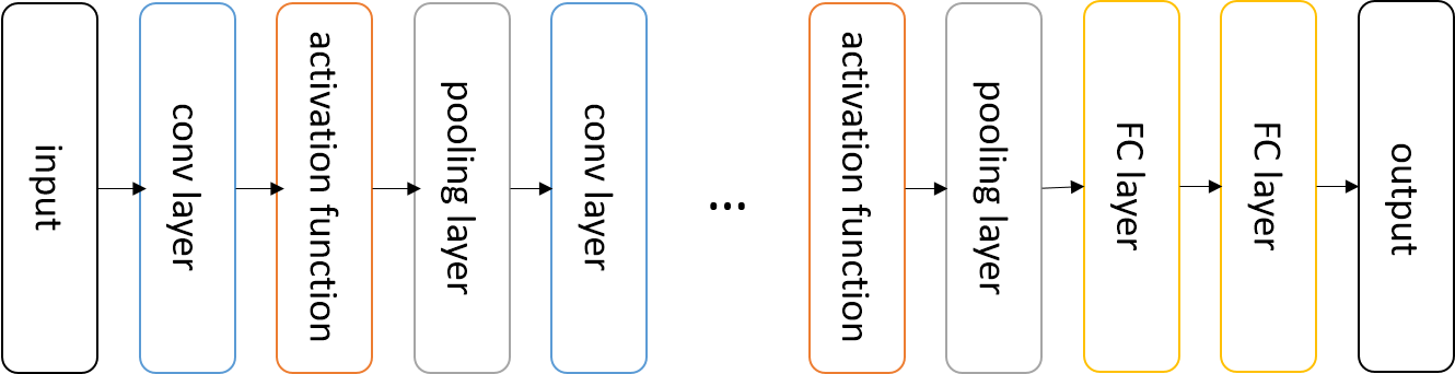
general architecture

• layer pattern

INPUT -> [ [CONV -> ACTIVATION] * N -> POOL? ] * M -> [ FC -> ACTIVATION ] * K -> FC?

Sometimes there is no pooling layers or FC layers.

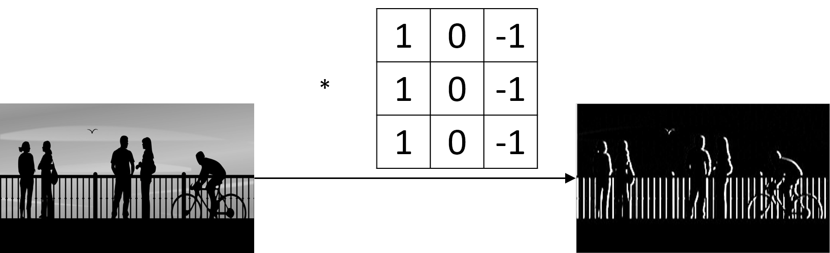
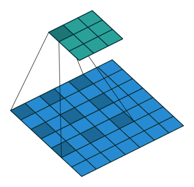
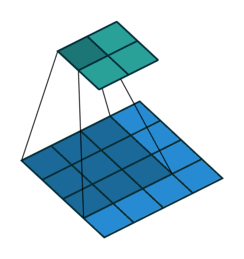
2.2. Convolutional Layer

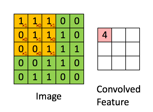
• A visualized impression of the convolution in the ConvNets

  

2.2.1. discrete convolution

• 1-D

  $$\begin{align*} s(t)=(x*w)(t)=\sum\limits_{a=-\infty}^{\infty}x(a)w(t-a) \tag{1} \end{align*}$$

  In convolutional network terminology, the first argument (in equation $(1)$, the function $x$) to the convolution is often referred to as the input, and the second argument (in equation $(1)$, the function $w$ ) as the kernel ( or filter ) . The output is sometimes referred to as the feature map.

• 2-D

  A two-dimensional image $I$ as input, a two-dimensional filter $K$.

  $$\begin{align*} S(i,j)=(I*K)(i,j)=\sum\limits_{m}\sum\limits_{n}I(m,n)K(i-m, j-n) \tag{2} \end{align*}$$

  The filter $K$ is flipped (We rotated it by 180 degrees along the center).

  

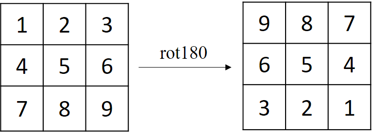
  So the equation $(2)$ is same as

  $$\begin{align*} S(i,j)=(I*K)(i,j)=\sum\limits_{m}\sum\limits_{n}I(i-m, j-n)K(m,n) \tag{3} \end{align*}$$

2.2.2. cross-correlation

The cross-correlation

$$\begin{align*} S(i,j)=(I*K)(i,j)=\sum\limits_{m}\sum\limits_{n}I(i+m,j+n)K(m, n) \tag{4} \end{align*}$$

We just do element-wise multiplies and sum over the results. No rotating.

• The two operations become interchangeable when the filter is learned (some trainable parameters).

• In practice,we usually use cross-correlation. But we also call it convolution by convention.

2.2.3. sparse connectivity

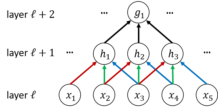
The unit $h_1$ only connects with units $\{x_1,x_2,x_3\}$.

• Each unit in a layer receives inputs from a set of units located in a small neighborhood in the previous. These units in the previous layer are called are known as the receptive field.

  e.g. The receptive field of $h_1$ is $\{x_1,x_2,x_3\}$.

• The units in the deeper layers can be indirectly connected to all or most of the input image.

• The idea of connecting units to local receptive fields on the inputs goes back to the Perceptron in the early 60s, and was almost simultaneous with Hubel and Wiesel's discovery of locally-sensitive, orientation-selective neurons in the cat's visual system.

  

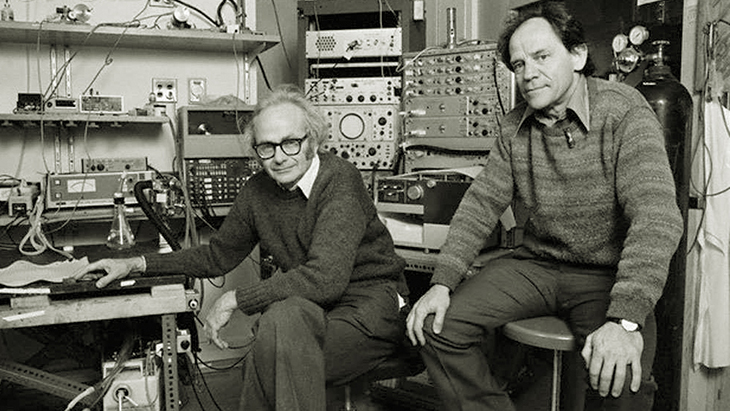
  David H. Hubel(left) and Torsten Wiesel(right)

2.2.4. parameter sharing

The edges between layer $\ell$ and layer $\ell+1$ with same colors have same weights.

• Each filter $K$ is replicated across the entire visual field. These replicated units share the same parameterization (weight vector and bias).

• Elementary feature detector that are useful on one part of the image are likely to be useful across the entire image.

  e.g. A vertical edge detector can detect vertical edges in the entire image.

  

• This can reduce a lot of parameters.

• The particular form of parameter sharing causes the layer to have a property called equivariance to translation. To say a function is equivariant means that if the input changes, the output changes in the same way. More details in chapter 9 of [5].

• In some cases, we may not wish to share parameters across the entire image. For example, if we are processing images that are cropped to be centered on an individual’s face, we probably want to extract different features at different locations.

2.2.5. padding

• valid convolution

  

  • In some open source code like tensorflow, if the size of input is $I\times I$, the filter's size is $K\times K$ and the stride is $S$, the size of output is $O\times O$, there is

    $$\begin{align*} O = \Big\lceil \frac{I-K+1}{S} \Big\rceil \tag{5} \end{align*}$$

  • Valid convolution will reduce the size of input.

  • When the layers go deeper, the pixels in the center will paly a more important role. You may lose information in the corners and edges.

• same convolution

  

  • If the size of input is $I\times I$, the zero-padding=$P$, the filter's size is $K\times K$ and the stride is $S$, the size of output is $O\times O$, there is

    $$\begin{align*} O = \Big\lfloor \frac{I+2P-K}{S} \Big\rfloor + 1 \tag{6} \end{align*}$$

  • In same convolution, more simplicity

  $$\begin{align*} O = \Big\lceil \frac{I}{S} \Big\rceil \tag{7} \end{align*}$$
  • This method helps us build deeper neural networks.

2.2.6. convolution over volume

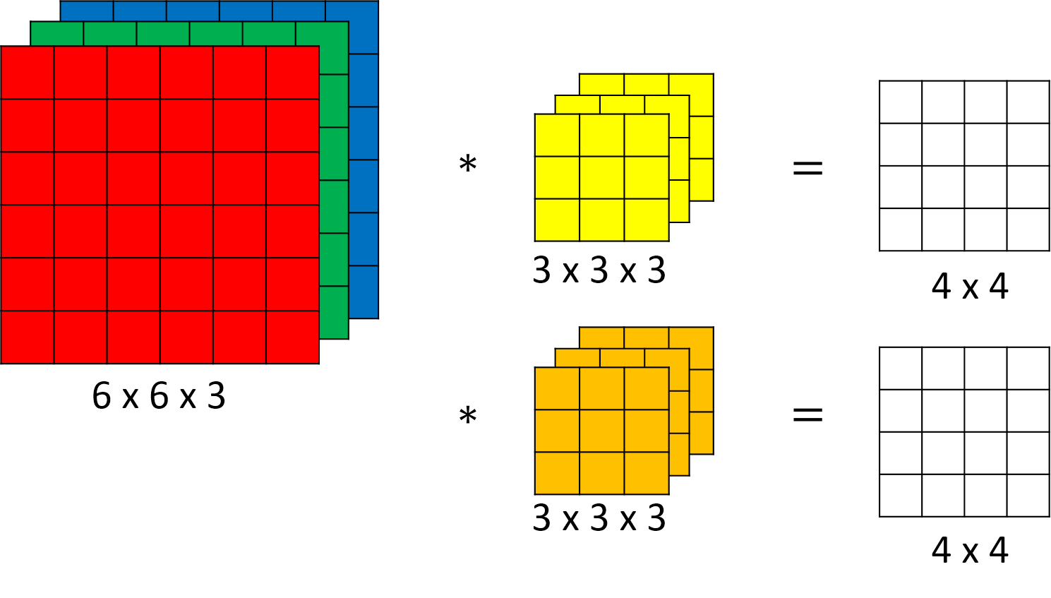
The picture is from [8].

• Natural images usually have multiple channels.

• The size of input volume is $H\times W \times C$, $C$ represents the channels' number.

  e.g. A RGB image haves 3 channels.

  The size of filter is $K\times K \times C$. Suppose there are $M$ filters. Stride = $1$.

  We do same convolution respectively.

  Then, the size of the output volume is $H \times W \times M$. The number of channels is $M$.

2.2.7. More...

• FC layers $\iff$ conv layers

  • converting FC layers to conv layers

    • The shape of input volume is $H\times W \times C$, the shape of filter is $H\times W \times C$. Then we can convert FC layers to conv layers.

  • converting conv layers to FC layers

    • We can set weights of the non-connected units between layer $\ell+1$ and layer $\ell$ to 0.
      Then we get a sparse weight matrix contains many zeros.

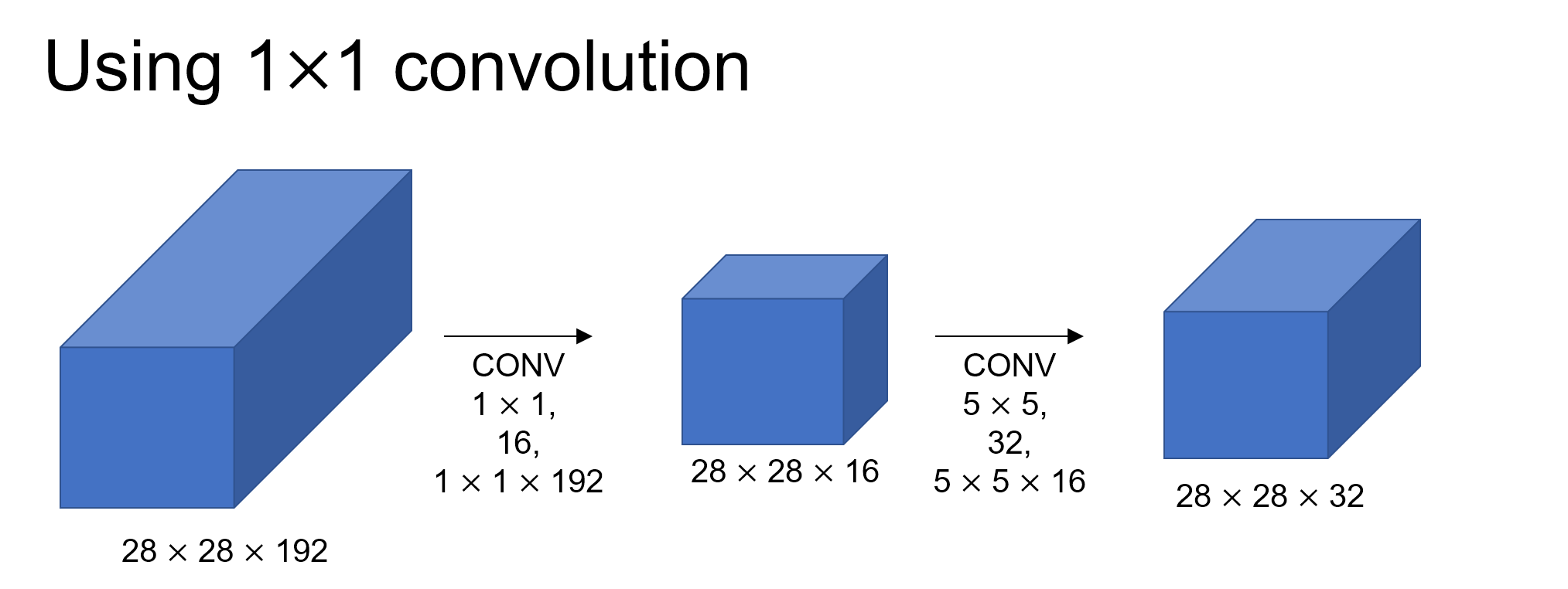
• 1x1 convolution

  • The shape of the filter is $1\times 1 \times C$.

  • This will help us to reduce the amount of computations and add more non-linearity.

  • consider the two cases(it is from [8])

    $$\begin{align*} 1.\ input(28\times28\times192) \rightarrow conv \ layer(5\times5\times192) \rightarrow output(28\times28 \times 32) \\ 2. \qquad \ \ \ input(28\times28\times192)\rightarrow conv \ layer (1\times1\times192)\rightarrow output(28\times28\times32) \\ \rightarrow conv \ layer(5\times5\times32)\rightarrow output(28\times28 \times 32) \end{align*}$$

    They have a huge difference in the number of multiplications.

  • The 1x1 convolution shrinks the number of channels sharply.In practice, it is tested that this method doesn't harm the performance of the network.

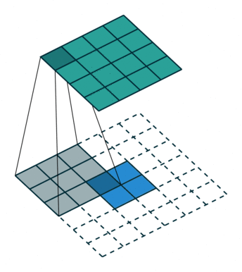
• dilated convolution

  

  The picture is from [4].

  • increasing the receptive field without decrease of spatial dimensions

• transposed convolution

  The need for transposed convolutions generally arises from the desire to use a transformation going in the opposite direction of a normal convolution.

  

  convolution

  

  transposed convolution

  The pictures are from [4].

  • You can see more in here or [4].

  • The filter was flipped vertically and horizontally.

  • It is called deconvolution in some literatures.

2.3. Activation Function

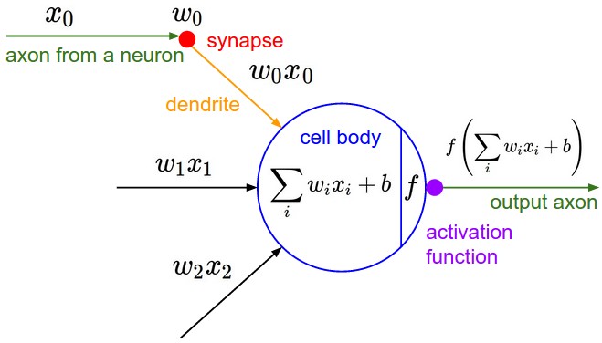
activation funciton

The picture is from [1].

• The activation function adds non-linearity to the network(some pooling methods also do this).

  A network without activation functions is just a linear mapping and cannot fit some complex functions.

2.3.1. sigmoid function

A sigmoid function is a mathematical function having a characteristic "S"-shaped curve or sigmoid curve. Often, sigmoid function refers to the special case of the logistic function shown in the figure and defined by the formula

$$\begin{align*} S(x) = \frac{1}{1+\exp(-x)} \tag{8} \end{align*}$$

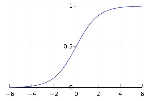
The picture is from wiki.

• logistic function

  $$\begin{align*} f(x) = \frac{L}{1+\exp(-k(x-x_0))} \tag{9} \end{align*}$$

• The gradient will be close to 0 when the value of the sigmoid function is close to 0 or 1. This phenomenon is called the "staturation effect" of the gradient.

  It will slow down the network's learning process.

2.3.2. rectifier

• the definition

  $$\begin{align*} f(x) = \max(0,x) \tag{10} \end{align*}$$

  A unit employing the rectifier is also called a rectified linear unit (ReLU ). For convention, we call the function ReLU.

  

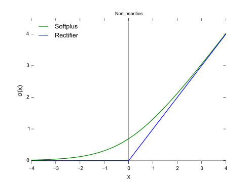
  The picture is from wiki.

• This is the most common activation function.

  ReLU can lead a faster learning rate than sigmoid function.

  ReLU performs pretty well in practice.

• There are some variants of ReLU in some literatures.

2.4. Pooling Layer

The role of the convolutional layer is to detect local conjunctions of features from the previous layer, the role of the pooling layer is to merge semantically similar features into one. [3]

• Not only is the precise position of each of those features irrelevant for identifying the pattern, it is potentially harmful because the position are likely to vary for different instances of the object.

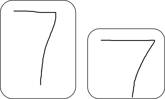
  • e.g. character 7 of different sizes

    We know that the input image contains the endpoint of a roughly horizontal segment in the upper left area, a corner in the upper right area, and the endpoint of a roughly vertical segment in the lower portion of the image, we can tell the input image is a 7.

    We do not care the size of the character most of the time.

• A simple way is to reduce the spatial resolution.

  It reduces the precision with which the position of distinctive features are encoded in a feature map.

  This can be achieved by pooling layers(sub-sampling layers).

2.4.1. max pooling

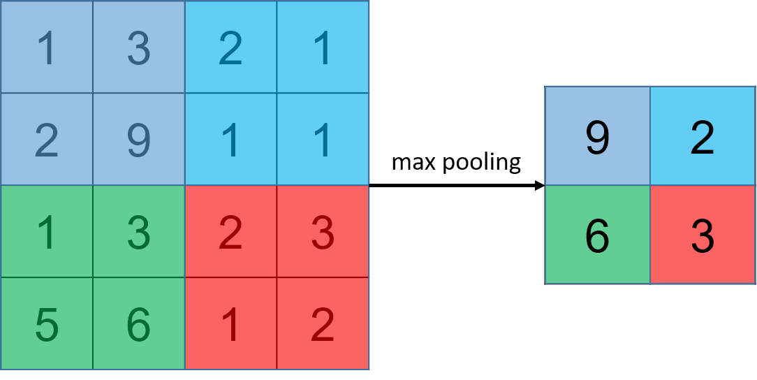
input : $4 \times 4$
pooling window : $2 \times 2$
stride : $2$
output : $2 \times 2$

• Max pooling get the max value of the units in the pooling window.

• In some open source code, there are "same" and "valid" pooling. The outputs' sizes are calculated in the same ways as "same" and "valid" convolution respectively.

2.4.2. average pooling

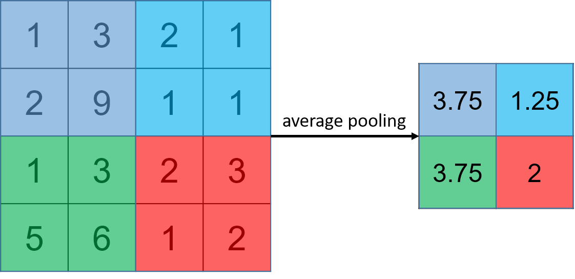
input : $4 \times 4$
pooling window : $2 \times 2$
stride : $2$
output : $2 \times 2$

• Average pooling caculate the average value of the units in the pooling window.

• Max pooling is more popular than average pooling in deep learning.

• If the input is volume, the pooling layer operates independently on every depth slice of the input and resizes it spatially.

• There are some other pooling methods like $\ell2$-norm pooling, you can search them by yourself.

3. Back-propagation

• It is the application of the chain rule.

  You may want to know about some knowledge of the vanilla back-propagation through fully connected networks. You can see [6]. A more detailed note is here.

• In vanilla back-propagation, the "error" propagating backwards through the network can be thought of as "sensitivities" of each unit with respect to perturbations of the bias.

• For simplicity, we do not consider about the activation function.

• notation

  • Superscript $[\ell]$ denotes an object of the $\ell$th layer.

    $\ell$th layer's next layer is $(\ell+1)$th layer, its previous layer is $(\ell-1)$th layer. $1 \le \ell \le L$.

    Layer $L$ is the output layer.

  • $n_H$, $n_W$ and $n_C$ denote respectively the height, width and number of channels of a given layer. If you want to reference a specific layer $\ell$, you can also write $n_H^{[\ell]}$, $n_W^{[\ell]}$, $n_C^{[\ell]}$.

  • We assume that each convolution layer $\ell$ is followed by a sub-sampling layer $\ell+1$.

3.1. convolution layers

For a certain filter $W_c^{\ell}$, its size is $f \times f \times n_C^{\ell-1}$ and the stride of convolution is $S$.

• computing the sensitivities

  • The key point is that sensitivities pass backward along the connected paths.

  • forward process

    $$\begin{align*} Z_c^{\ell} = \text{conv}(A^{\ell}, \ W_c^{\ell}, \ \text{stride}=S) \tag{11} \end{align*}$$

    Where $\text{conv}(\cdot)$ denotes a convolution operation.

    The shape of the input $A^{\ell}$ is $n_H^{[\ell-1]} \times n_W^{[\ell-1]} \times n_C^{[\ell-1]}$, the shape of the output $Z_c^{\ell}$ is $n_H^{[\ell]} \times n_W^{[\ell]}$.

    The shape of sensitivities $\delta^{\ell}$ is $n_H^{[\ell]} \times n_W^{[\ell]} \times n_C^{[\ell]}$.
    The shape of sensitivities $\delta^{\ell-1}$ is $n_H^{[\ell-1]} \times n_W^{[\ell-1]} \times n_C^{[\ell-1]}$.
    The shape of $W_c^{\ell}$ is $f\times f \times n_C^{[\ell-1]}$.

    The output of the $(\ell-1)$th is equal to the input of the $\ell$th layer.

    For the element $Z_{hwc}^{\ell}$

    $$\begin{align*} Z_{hwc}^{\ell} = \text{reduce_sum}( A_{slice} \circ W_c^{\ell} ) + b_c^{\ell} \tag{12} \end{align*}$$

    Where $\text{reduce_sum}( \cdot )$ denotes an operation that computes the sum of the matrix's elements, the operator $\circ$ denotes element-wise multiplication.
    $A_{slice}^{\ell}$ corresponds to the slice which was used to generate the acitivation $Z_{hwc}^{\ell}$.
    The shape of $A_{slice}^{\ell}$ is $f\times f \times n_C^{[\ell-1]}$, it's same as the shape of $W_c^{\ell}$.

    $$\begin{align*} A_{slice}^{\ell} = A^{\ell}[i:i+f,\ j:j+f, \ :] \tag{13} \end{align*}$$

    Where $i = h \times S$, $j = w \times S$.

  • backpropagation

  $$\begin{align*} \delta^{\ell-1}[i:i+f,\ j:j+f, \ :] \ = \sum_cW_c^{\ell} \times \delta^{\ell}_{hwc} \tag{14} \end{align*}$$

  Where $i = h \times S$, $j = w \times S$, and $\delta^{\ell}_{hwc}$ is a scalar corresponding to the gradient of the cost with respect to the output of the conv layer $\ell$ at the $h$th row, $w$th column and $c$th channel.
  In fact, this can be achieved by a convolutional operation. You can see [6] for more details.

  • At each time, we multiply the the same filter $W_c^{\ell}$ by a different $\delta^{\ell}_{hwc}$ when updating sensitivities. We can get the final $\delta^{\ell-1}$ by iterating $h$,$w$ and $c$.

  • We do so mainly because when computing the forward propagation, each filter is dotted and summed by a different $A_{slice}^{\ell}$. Therefore when computing the backprop for dA, we are just adding the gradients of all the $A_{slice}^{\ell}$s.

• Computing $\text{d}W$

  This is the formula for computing $\text{d}W_c^{\ell}$ with respect to the loss:

  $$\begin{align*} \text{d}W_c^{\ell} = \sum _{h=0} ^{n_H} \sum_{w=0} ^ {n_W} A_{slice}^{\ell} \times \delta^{\ell}_{hwc} \tag{15} \end{align*}$$

  This ends up giving us the gradient for $W_c^{\ell}$ with respect to that slice. Since it is the same $W_c^{\ell}$, we will just add up all such gradients to get $\text{d}W_c^{\ell}$.

• Computing $\text{d}b$:

  This is the formula for computing $\text{d}b_c^{\ell}$ with respect to the cost for a certain filter $W_c^{\ell}$:

  $$\begin{align*} \text{d}b_c^{\ell} = \sum _{h=0} ^{n_H} \sum_{w=0} ^ {n_W} \delta^{\ell}_{hwc} \tag{16} \end{align*}$$

  As we have previously seen in basic neural networks, $\text{d}b$ is computed by summing sensitivities. In this case, we are just summing over all the gradients of the conv output ($Z^{\ell}$) with respect to the cost.

3.3. pooling Layer

A pooling layer has no parameters for backprop to update, we still need to backprop the gradient through the pooling layer in order to compute gradients for layers that came before the pooling layer.

If the size of the pooling window is $f \times f$ and the stride of pooling is $S$.

• forward process

  $$\begin{align*} Z_c^{\ell} = \text{pool}(A_c^{\ell}, \ \text{size}=[f,f], \ \text{stride}=S) \tag{17} \end{align*}$$

  Where $\text{pool}(\cdot)$ denotes a pooling operation.

  The shape of the input slice $A_c^{\ell}$ is $n_H^{[\ell-1]} \times n_W^{[\ell-1]}$, the shape of the output $Z_c^{\ell}$ is $n_H^{[\ell]} \times n_W^{[\ell]}$.

  The shape of sensitivities $\delta^{\ell}$ is $n_H^{[\ell]} \times n_W^{[\ell]} \times n_C^{[\ell]}$.
  The shape of sensitivities $\delta^{\ell-1}$ is $n_H^{[\ell-1]} \times n_W^{[\ell-1]} \times n_C^{[\ell-1]}$.

  $n_C^{[\ell-1]} = n_C^{[\ell]}$.

• max pooling

  We need keeps track of where the index of the maximum of input. Only the maximum contribute to the backpropagation. Suppose $f=2$

  $$\begin{align*} X = \begin{bmatrix} 1 && 3 \\ 4 && 2 \end{bmatrix} \quad \rightarrow \quad M =\begin{bmatrix} 0 && 0 \\ 1 && 0 \end{bmatrix}\tag{18} \end{align*}$$

  A "mask" matrix which True (1) indicates the position of the maximum in X, the other entries are False (0).

• average pooliing

  In max pooling, for each input window, all the "influence" on the output came from a single input value--the max.

  In average pooling, every element of the input window has equal influence on the output.

  Suppose $f=2$, then the mask we'll use for the backward pass will look like:
  

  $$\begin{align*} M =\begin{bmatrix} 1/4 && 1/4 \\ 1/4 && 1/4 \end{bmatrix} \tag{19} \end{align*}$$

  This implies that each position in the $\delta$ matrix contributes equally to output because in the forward pass, we took an average.

• backpropagation

  $$\begin{align*} \delta^{\ell-1}{[i:i+f,\ j:j+f, \ c]} \ = M \times \delta^{\ell}_{hwc} \tag{20} \end{align*}$$

  Where $i = h \times S$, $j = w \times S$, and $\delta^{\ell}_{hwc}$ is a scalar corresponding to the gradient of the cost with respect to the output of the conv layer $\ell$ at the $h$th row, $w$th column and $c$th channel.

4. Case studies

4.1. LeNet-5

• The first successful applications of Convolutional Networks were developed by Yann LeCun in 1990's.

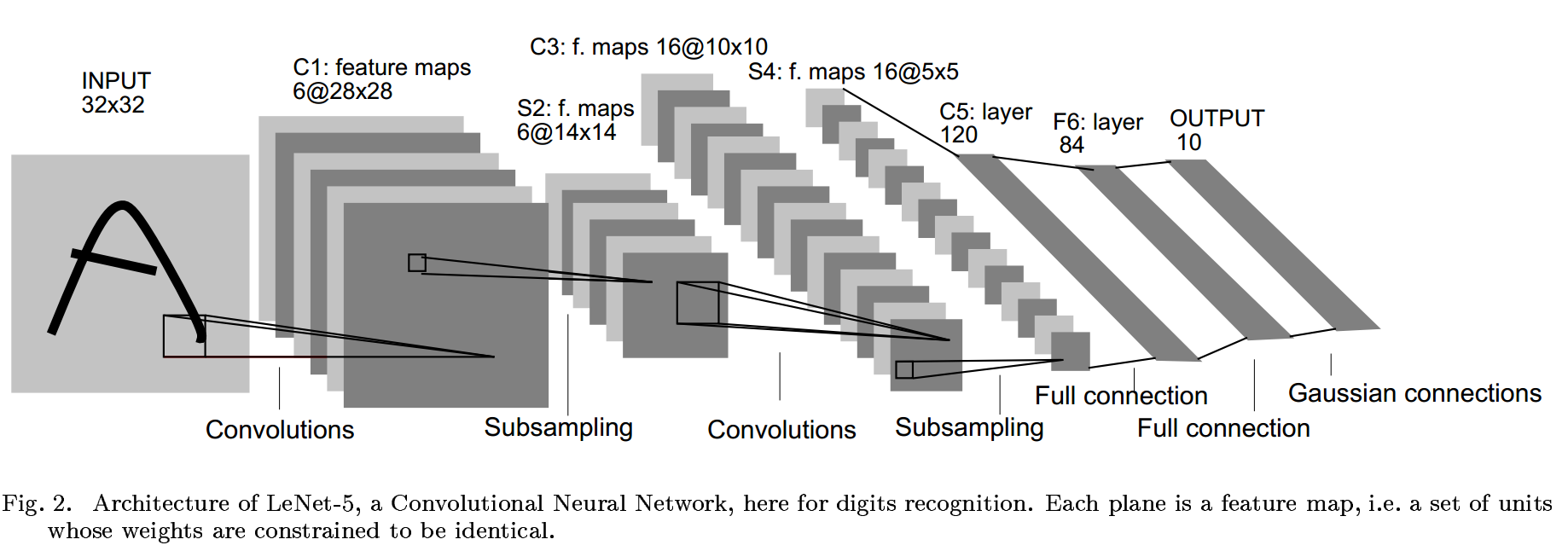
The picture is from [7].

• LeNet-5 comprises 7 layers, not counting the input, all of which contain trainable parameters. Convolutional layers are labeled $Cx$, sub-sampling layers are labeled $Sx$, and FC layers are labeled $Fx$.

• The sizes of the convolutional filters are all $5 \times 5$. LeNet-5 uses average pooling. After getting the average value, it will be multiplied by a trainable coefficient and added to a trainble bias. Be careful that the feature map in $C3$ is not connected to every feature $S2$ feature map.

• The output layer is composed of Euclidean Radial Basis Function units(RBF).You can see more details in [7].

• There are also LeNet-1 and LeNet-4 in [7]. Their architectures are similar.

Yann LeCun

4.2. AlexNet

• The first work that popularized Convolutional Networks in Computer Vision.

  The winner of ILSVRC 2012.

  

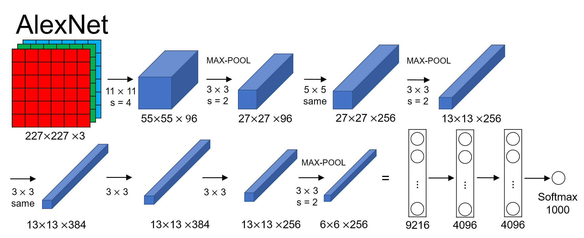
  The picture is from [8].

  • There are about 60M trainable parameters in the AlexNet.

  • It seems different from the picture in the [9]. In fact, they are same . About the sofmax, you can see here.

  • It's named after the author Alex Krizhevsky. More details in [9].

4.3. VGGNet

• The runner-up of ILSVRC 2014.

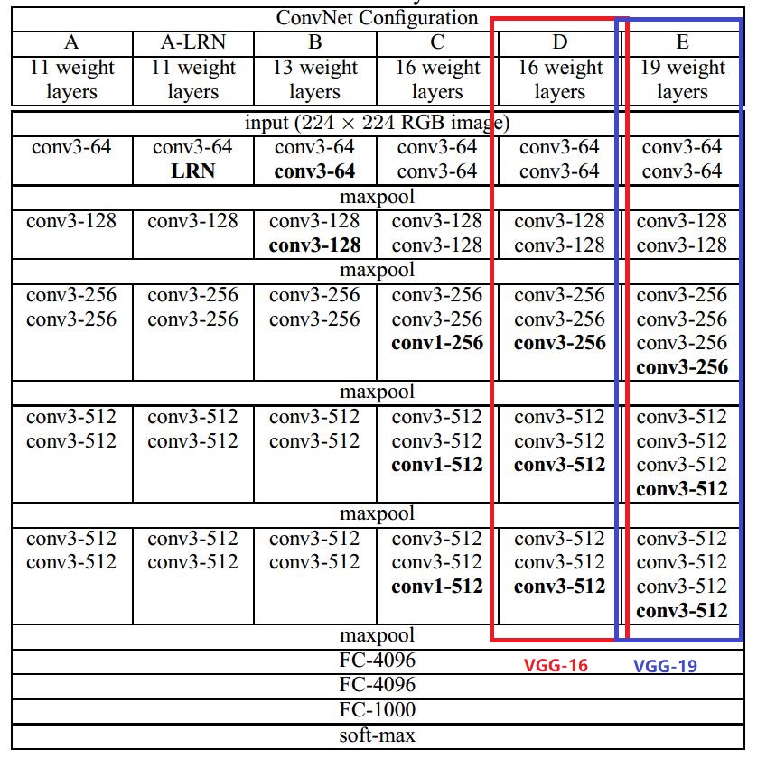
The picture is from [10].

• The paper [10] is from Visual Geometry Group in University of Oxford.

• The size of pooling window is 2x2. The convolutional layer parameters are denoted as "conv$<$receptive field size$>$ $-$ $<$number of channels$>$". They are all same convolutions. You can see that sizes of all the filters are 3x3. The use of small convolutional filter can reduce the amount of parameters.

  e.g. a single 7x7 conv. layer and a stack of three 3x3 conv. layers. They all have 7x7 effective receptive. Suppose they all have $C$ channels.
  The former need $7^2C^2=49C^2$ parameters, the latter need $3(3^2C^2)=27C^2$ parameters.

• The VGG-16 is used most commonly. It is as well as the VGG-19 according to the experiments in [10].They both perform better than other ConvNets in the table in the experiments. More details in [10].

4.4. Inception

The ILSVRC 2014 winner.

• motivation

  When we design a layer for a ConvNet, we may consider about the 1x1 conv. filter, 3x3 conv. filter , 5x5 conv. filter, or we want a pooling layer. Why not do them all?

• inception module

  

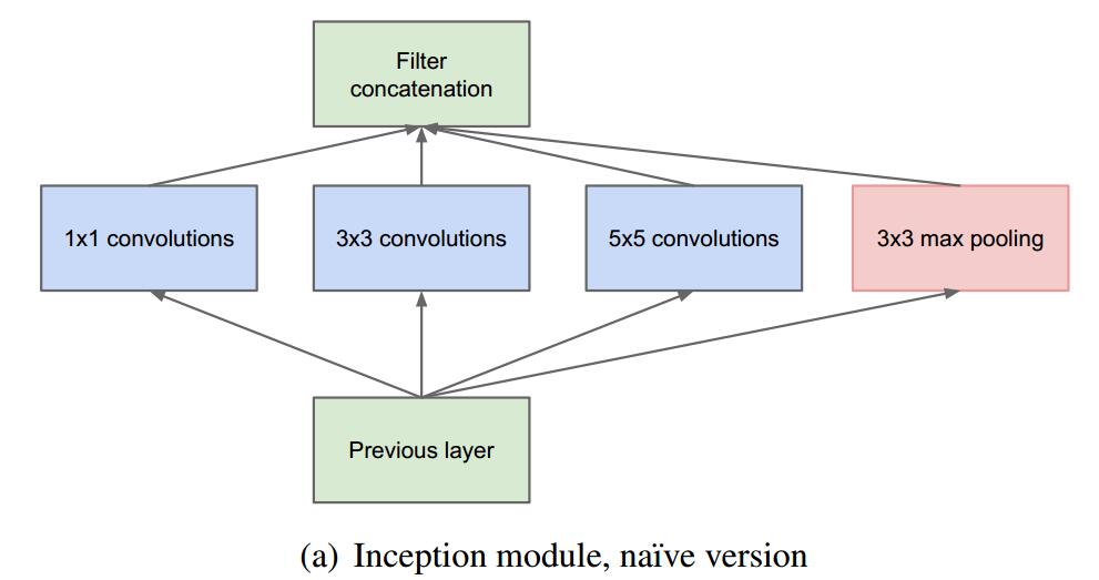
  The picture is from [11].

  naive verison of inception module

  

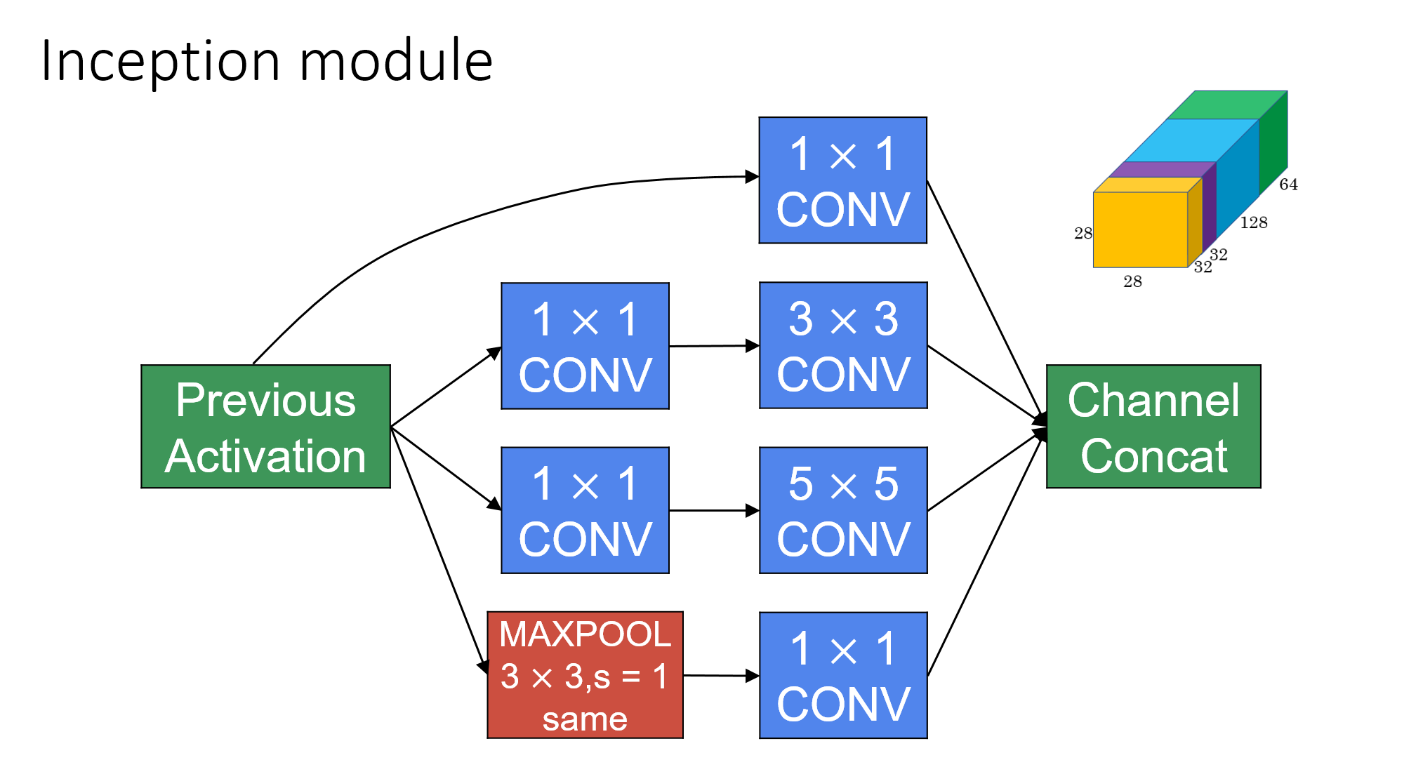
  inception module with dimensionality reduction

  The pictures are from [8]

  • Dimensionality reduction can help us reduce the amount of computations.

    

• GoogLeNet

  • The "GoogLeNet" name refer to the particular incarnation of the Inception architecture used in the ILSVRC 2014 competition. It is a stack of many inception modules.

  

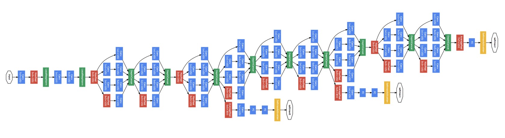
  GooLeNet

  The picture is fuzzy. You can find the original one in [11].

  • There are also Inception V2, Inception V3 and Inception V4. You can search them by yourself.

4.5. ResNet

• The winner of ILSVRC 2015.

• Is learning better networks as easy as stacking more layers?

  • The main benefit of a very deep network is that it can represent very complex functions. It can also learn features at many different levels of abstraction.

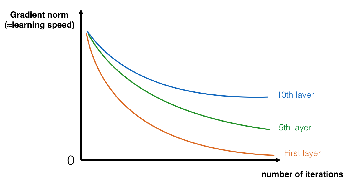
  • A huge barrier to training deep network is vanishing gradients.

    During gradient descent, as you backprop from the final layer back to the first layer, you are multiplying by the weight matrix on each step, and thus the gradient can decrease exponentially quickly to zero (or, in rare cases, grow exponentially quickly and "explode" to take very large values).

    

    The picture is from [8].

  • When deeper networks are able to start converging, a degradation problem has been exposed: with the network depth increasing, accuracy gets saturated and then degrades rapidly.

    

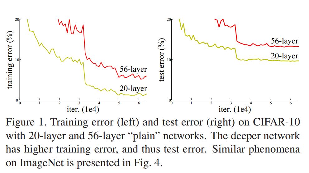
    The picture is from [12].

• residual block

  

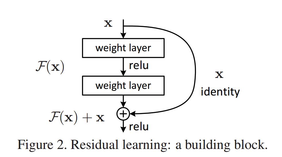
  The picture is from [12].

  • The formulation of $\mathcal{F}(x)+x$ can be realized by feedforward nerral networks with "shortcut connections".

    The output of the block is $\mathbf{y}$ (before ReLU).

    $$\begin{align*} \mathbf{y} = \mathcal{F}(\mathbf{x}, {W_i}) + \mathbf{x} \tag{11} \end{align*}$$

    $\mathcal{F}(\mathbf{x}, {W_i})$ represents the residual mapping to be learned. There are two layers in the picture. $\mathcal{F} = W_2\sigma(W_1 \mathbf{x})$, in which $\sigma$ denotes ReLU and the biases are ommitted for simplicity.

  • Be careful that the dimensions of $\mathbf{x}$ and $\mathcal{F}$ must be equal.

  • This really helps with the vanishing and exploding gradient problems and allows us to train much deeper neural networks without really appreciable loss in performance.

    There are ResNet-34, ResNet-50, ResNet-101 and ResNet-152 in [12].

    More details in [12].

Reference

[1] http://cs231n.github.io/convolutional-networks/#conv

[2] http://ufldl.stanford.edu/tutorial/supervised/FeatureExtractionUsingConvolution/

[3] Y. LeCun, Y. Bengio, G. Hinton. (2015). Deep learning.

[4] D. Vincent, V. Francesco. (2016). A guide to convolution arithmetic for deep learning.

[5] I. Goodfellow, Y. Bengio, and A. Courville. (2016). Deep learning. Book in preparation for MIT Press.

[6] J. Bouvrie. Notes on Convolutional Neural Networks.

[7] Y. LeCun, L. Bottou, Y. Bengio, and P. Haffner. (1998). Gradient-based learning applied to document recognition.

[8] https://www.coursera.org/learn/convolutional-neural-networks/

[9] A. Krizhevsky, I. Sutskever, G. E. Hinton. (2012). ImageNet classification with deep convolutional neural networks.

[10] K. Simonyan, A. Zisserman. (2015). Very deep convolutional networks for large-scale image recognition.

[11] C.Szegedy, W. Liu, Y. Jia, P. Sermanet et al. (2015). Going deeper with convolutions.

[12] K. He, X. Zhang, S. Ren, J. Sun. (2016). Deep residual learning for image recognition.

Log

• 2017.12.31 正式完成基本内容。

• 2018.01.15 修改部分关于神经网络中反向传播的内容。

• 2018.01.18 小改。

Other

Contact Me : 1696144426@qq.com

All contents Copyright 2017. All rights reserved.