week03.Ng's Sequence Model Course-Homework

2018.02 Coursera

---

Neural Machine Translation

Welcome to your first programming assignment for this week!

You will build a Neural Machine Translation (NMT) model to translate human readable dates ("25th of June, 2009") into machine readable dates ("2009-06-25"). You will do this using an attention model, one of the most sophisticated sequence to sequence models.

This notebook was produced together with NVIDIA's Deep Learning Institute.

Let's load all the packages you will need for this assignment.

from keras.layers import Bidirectional, Concatenate, Permute, Dot, Input, LSTM, Multiply
from keras.layers import RepeatVector, Dense, Activation, Lambda
from keras.optimizers import Adam
from keras.utils import to_categorical
from keras.models import load_model, Model
import keras.backend as K
import numpy as np
from faker import Faker
import random
from tqdm import tqdm
from babel.dates import format_date
from nmt_utils import *
import matplotlib.pyplot as plt
%matplotlib inline

1 - Translating human readable dates into machine readable dates

The model you will build here could be used to translate from one language to another, such as translating from English to Hindi. However, language translation requires massive datasets and usually takes days of training on GPUs. To give you a place to experiment with these models even without using massive datasets, we will instead use a simpler "date translation" task.

The network will input a date written in a variety of possible formats (e.g. "the 29th of August 1958", "03/30/1968", "24 JUNE 1987") and translate them into standardized, machine readable dates (e.g. "1958-08-29", "1968-03-30", "1987-06-24"). We will have the network learn to output dates in the common machine-readable format YYYY-MM-DD.

1.1 - Dataset

We will train the model on a dataset of 10000 human readable dates and their equivalent, standardized, machine readable dates. Let's run the following cells to load the dataset and print some examples.

m = 10000
dataset, human_vocab, machine_vocab, inv_machine_vocab = load_dataset(m)

dataset[:10]
result：
[('9 may 1998', '1998-05-09'),
 ('10.09.70', '1970-09-10'),
 ('4/28/90', '1990-04-28'),
 ('thursday january 26 1995', '1995-01-26'),
 ('monday march 7 1983', '1983-03-07'),
 ('sunday may 22 1988', '1988-05-22'),
 ('tuesday july 8 2008', '2008-07-08'),
 ('08 sep 1999', '1999-09-08'),
 ('1 jan 1981', '1981-01-01'),
 ('monday may 22 1995', '1995-05-22')]

You've loaded:
- dataset: a list of tuples of (human readable date, machine readable date)
- human_vocab: a python dictionary mapping all characters used in the human readable dates to an integer-valued index
- machine_vocab: a python dictionary mapping all characters used in machine readable dates to an integer-valued index. These indices are not necessarily consistent with human_vocab.
- inv_machine_vocab: the inverse dictionary of machine_vocab, mapping from indices back to characters.

Let's preprocess the data and map the raw text data into the index values. We will also use Tx=30 (which we assume is the maximum length of the human readable date; if we get a longer input, we would have to truncate it) and Ty=10 (since "YYYY-MM-DD" is 10 characters long).

Tx = 30
Ty = 10
X, Y, Xoh, Yoh = preprocess_data(dataset, human_vocab, machine_vocab, Tx, Ty)
print("X.shape:", X.shape)
print("Y.shape:", Y.shape)
print("Xoh.shape:", Xoh.shape)
print("Yoh.shape:", Yoh.shape)
result:
X.shape: (10000, 30)
Y.shape: (10000, 10)
Xoh.shape: (10000, 30, 37)
Yoh.shape: (10000, 10, 11)

You now have:
- X: a processed version of the human readable dates in the training set, where each character is replaced by an index mapped to the character via human_vocab. Each date is further padded to $T_x$ values with a special character (< pad >). X.shape = (m, Tx)
- Y: a processed version of the machine readable dates in the training set, where each character is replaced by the index it is mapped to in machine_vocab. You should have Y.shape = (m, Ty).
- Xoh: one-hot version of X, the "1" entry's index is mapped to the character thanks to human_vocab. Xoh.shape = (m, Tx, len(human_vocab))
- Yoh: one-hot version of Y, the "1" entry's index is mapped to the character thanks to machine_vocab. Yoh.shape = (m, Tx, len(machine_vocab)). Here, len(machine_vocab) = 11 since there are 11 characters ('-' as well as 0-9).

Lets also look at some examples of preprocessed training examples. Feel free to play with index in the cell below to navigate the dataset and see how source/target dates are preprocessed.

index = 0
print("Source date:", dataset[index][0])
print("Target date:", dataset[index][1])
print()
print("Source after preprocessing (indices):", X[index])
print("Target after preprocessing (indices):", Y[index])
print()
print("Source after preprocessing (one-hot):", Xoh[index])
print("Target after preprocessing (one-hot):", Yoh[index])
result:
Source date: 9 may 1998
Target date: 1998-05-09
Source after preprocessing (indices): [12  0 24 13 34  0  4 12 12 11 36 36 36 36 36 36 36 36 36 36 36 36 36 36 36
 36 36 36 36 36]
Target after preprocessing (indices): [ 2 10 10  9  0  1  6  0  1 10]
Source after preprocessing (one-hot): [[ 0.  0.  0. ...,  0.  0.  0.]
 [ 1.  0.  0. ...,  0.  0.  0.]
 [ 0.  0.  0. ...,  0.  0.  0.]
 ..., 
 [ 0.  0.  0. ...,  0.  0.  1.]
 [ 0.  0.  0. ...,  0.  0.  1.]
 [ 0.  0.  0. ...,  0.  0.  1.]]
Target after preprocessing (one-hot): [[ 0.  0.  1.  0.  0.  0.  0.  0.  0.  0.  0.]
 [ 0.  0.  0.  0.  0.  0.  0.  0.  0.  0.  1.]
 [ 0.  0.  0.  0.  0.  0.  0.  0.  0.  0.  1.]
 [ 0.  0.  0.  0.  0.  0.  0.  0.  0.  1.  0.]
 [ 1.  0.  0.  0.  0.  0.  0.  0.  0.  0.  0.]
 [ 0.  1.  0.  0.  0.  0.  0.  0.  0.  0.  0.]
 [ 0.  0.  0.  0.  0.  0.  1.  0.  0.  0.  0.]
 [ 1.  0.  0.  0.  0.  0.  0.  0.  0.  0.  0.]
 [ 0.  1.  0.  0.  0.  0.  0.  0.  0.  0.  0.]
 [ 0.  0.  0.  0.  0.  0.  0.  0.  0.  0.  1.]]

2 - Neural machine translation with attention

If you had to translate a book's paragraph from French to English, you would not read the whole paragraph, then close the book and translate. Even during the translation process, you would read/re-read and focus on the parts of the French paragraph corresponding to the parts of the English you are writing down.

The attention mechanism tells a Neural Machine Translation model where it should pay attention to at any step.

2.1 - Attention mechanism

In this part, you will implement the attention mechanism presented in the lecture videos. Here is a figure to remind you how the model works. The diagram on the left shows the attention model. The diagram on the right shows what one "Attention" step does to calculate the attention variables $\alpha^{\langle t, t' \rangle}$, which are used to compute the context variable $context^{\langle t \rangle}$ for each timestep in the output ($t=1, \ldots, T_y$).

Figure 1: Neural machine translation with attention

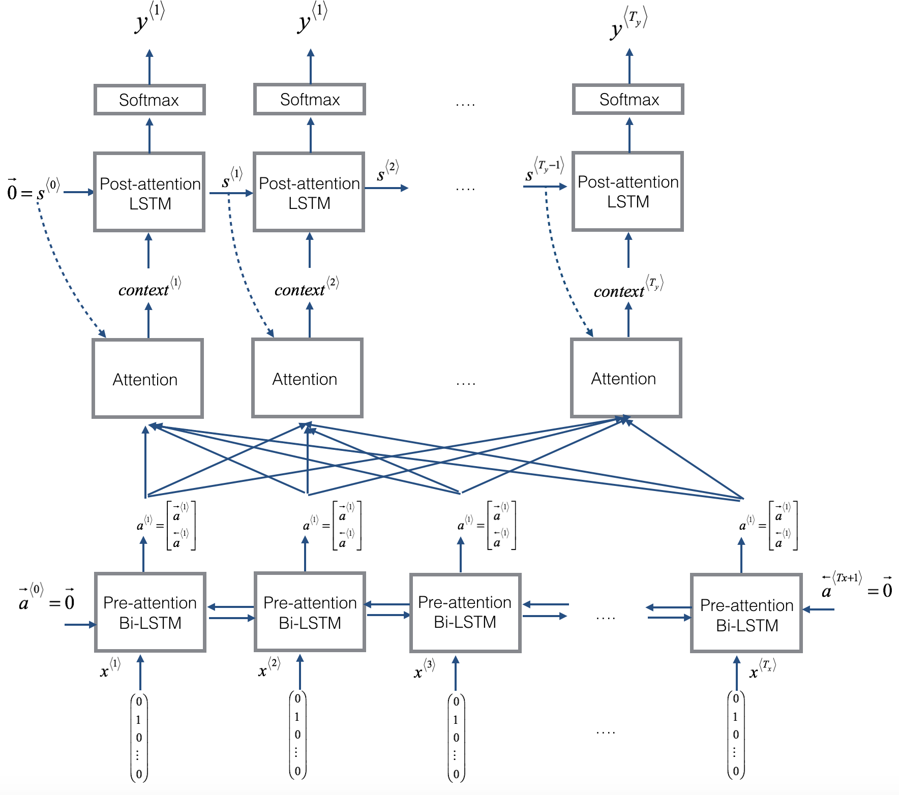
Here are some properties of the model that you may notice:

• There are two separate LSTMs in this model (see diagram on the left). Because the one at the bottom of the picture is a Bi-directional LSTM and comes before the attention mechanism, we will call it pre-attention Bi-LSTM. The LSTM at the top of the diagram comes after the attention mechanism, so we will call it the post-attention LSTM. The pre-attention Bi-LSTM goes through $T_x$ time steps; the post-attention LSTM goes through $T_y$ time steps.

• The post-attention LSTM passes $s^{\langle t \rangle}, c^{\langle t \rangle}$ from one time step to the next. In the lecture videos, we were using only a basic RNN for the post-activation sequence model, so the state captured by the RNN output activations $s^{\langle t\rangle}$. But since we are using an LSTM here, the LSTM has both the output activation $s^{\langle t\rangle}$ and the hidden cell state $c^{\langle t\rangle}$. However, unlike previous text generation examples (such as Dinosaurus in week 1), in this model the post-activation LSTM at time $t$ does will not take the specific generated $y^{\langle t-1 \rangle}$ as input; it only takes $s^{\langle t\rangle}$ and $c^{\langle t\rangle}$ as input. We have designed the model this way, because (unlike language generation where adjacent characters are highly correlated) there isn't as strong a dependency between the previous character and the next character in a YYYY-MM-DD date.

  注意与post-attention LSTM模块与text generation model的不同之处，并没有利用前一个time step的输出$y^{<t-1>}$作为后一个time step的输入。

• We use $a^{\langle t \rangle} = [\overrightarrow{a}^{\langle t \rangle}; \overleftarrow{a}^{\langle t \rangle}]$ to represent the concatenation of the activations of both the forward-direction and backward-directions of the pre-attention Bi-LSTM.

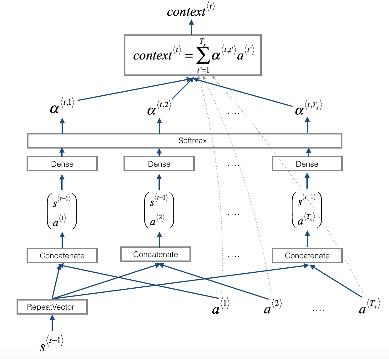
• The diagram on the right uses a RepeatVector node to copy $s^{\langle t-1 \rangle}$'s value $T_x$ times, and then Concatenation to concatenate $s^{\langle t-1 \rangle}$ and $a^{\langle t \rangle}$ to compute $e^{\langle t, t'}$, which is then passed through a softmax to compute $\alpha^{\langle t, t' \rangle}$. We'll explain how to use RepeatVector and Concatenation in Keras below.

Lets implement this model. You will start by implementing two functions: one_step_attention() and model().

1) one_step_attention(): At step $t$, given all the hidden states of the Bi-LSTM ($[a^{<1>},a^{<2>}, ..., a^{<T_x>}]$) and the previous hidden state of the second LSTM ($s^{<t-1>}$), one_step_attention() will compute the attention weights ($[\alpha^{<t,1>},\alpha^{<t,2>}, ..., \alpha^{<t,T_x>}]$) and output the context vector (see Figure 1 (right) for details):

$$context^{<t>} = \sum_{t' = 0}^{T_x} \alpha^{<t,t'>}a^{<t'>}\tag{1}$$

Note that we are denoting the attention in this notebook $context^{\langle t \rangle}$. In the lecture videos, the context was denoted $c^{\langle t \rangle}$, but here we are calling it $context^{\langle t \rangle}$ to avoid confusion with the (post-attention) LSTM's internal memory cell variable, which is sometimes also denoted $c^{\langle t \rangle}$.

2) model(): Implements the entire model. It first runs the input through a Bi-LSTM to get back $[a^{<1>},a^{<2>}, ..., a^{<T_x>}]$. Then, it calls one_step_attention() $T_y$ times (for loop). At each iteration of this loop, it gives the computed context vector $c^{<t>}$ to the second LSTM, and runs the output of the LSTM through a dense layer with softmax activation to generate a prediction $\hat{y}^{<t>}$.

Exercise: Implement one_step_attention(). The function model() will call the layers in one_step_attention() $T_y$ using a for-loop, and it is important that all $T_y$ copies have the same weights. I.e., it should not re-initiaiize the weights every time. In other words, all $T_y$ steps should have shared weights. Here's how you can implement layers with shareable weights in Keras:
1. Define the layer objects (as global variables for examples).
2. Call these objects when propagating the input.

We have defined the layers you need as global variables. Please run the following cells to create them. Please check the Keras documentation to make sure you understand what these layers are: RepeatVector(), Concatenate(), Dense(), Activation(), Dot().

# Defined shared layers as global variables
repeator = RepeatVector(Tx)
concatenator = Concatenate(axis=-1)
densor1 = Dense(10, activation = "tanh")
densor2 = Dense(1, activation = "relu")
activator = Activation(softmax, name='attention_weights') # We are using a custom softmax(axis = 1) loaded in this notebook
dotor = Dot(axes = 1)

Now you can use these layers to implement one_step_attention(). In order to propagate a Keras tensor object X through one of these layers, use layer(X) (or layer([X,Y]) if it requires multiple inputs.), e.g. densor(X) will propagate X through the Dense(1) layer defined above.

# GRADED FUNCTION: one_step_attention
def one_step_attention(a, s_prev):
    """
    Performs one step of attention: Outputs a context vector computed as a dot product of the attention weights
    "alphas" and the hidden states "a" of the Bi-LSTM.
    Arguments:
    a -- hidden state output of the Bi-LSTM, numpy-array of shape (m, Tx, 2*n_a)
    s_prev -- previous hidden state of the (post-attention) LSTM, numpy-array of shape (m, n_s)
    Returns:
    context -- context vector, input of the next (post-attetion) LSTM cell
    """
    ### START CODE HERE ###
    # m, Tx, na_2 = a.shape
    # Use repeator to repeat s_prev to be of shape (m, Tx, n_s) so that you can concatenate it with all hidden states "a" (≈ 1 line)
    s_prev = repeator(s_prev)
    # Use concatenator to concatenate a and s_prev on the last axis (≈ 1 line)
    concat = concatenator([a, s_prev])
    # Use densor1 to propagate concat through a small fully-connected neural network to compute the "intermediate energies" variable e. (≈1 lines)
    e = densor1(concat)
    # Use densor2 to propagate e through a small fully-connected neural network to compute the "energies" variable energies. (≈1 lines)
    energies = densor2(e)
    # Use "activator" on "energies" to compute the attention weights "alphas" (≈ 1 line)
    alphas = activator(energies)
    # Use dotor together with "alphas" and "a" to compute the context vector to be given to the next (post-attention) LSTM-cell (≈ 1 line)
    context = dotor([alphas, a])
    ### END CODE HERE ###
    return context

You will be able to check the expected output of one_step_attention() after you've coded the model() function.

Exercise: Implement model() as explained in figure 2 and the text above. Again, we have defined global layers that will share weights to be used in model().

n_a = 32
n_s = 64
post_activation_LSTM_cell = LSTM(n_s, return_state = True)
output_layer = Dense(len(machine_vocab), activation=softmax)

Now you can use these layers $T_y$ times in a for loop to generate the outputs, and their parameters will not be reinitialized. You will have to carry out the following steps:

1. Propagate the input into a Bidirectional LSTM

2. Iterate for $t = 0, \dots, T_y-1$:

   1. Call one_step_attention() on $[\alpha^{<t,1>},\alpha^{<t,2>}, ..., \alpha^{<t,T_x>}]$ and $s^{<t-1>}$ to get the context vector $context^{<t>}$.
   2. Give $context^{<t>}$ to the post-attention LSTM cell. Remember pass in the previous hidden-state $s^{\langle t-1\rangle}$ and cell-states $c^{\langle t-1\rangle}$ of this LSTM using initial_state= [previous hidden state, previous cell state]. Get back the new hidden state $s^{<t>}$ and the new cell state $c^{<t>}$.
   3. Apply a softmax layer to $s^{<t>}$, get the output.
   4. Save the output by adding it to the list of outputs.

3. Create your Keras model instance, it should have three inputs ("inputs", $s^{<0>}$ and $c^{<0>}$) and output the list of "outputs".

# GRADED FUNCTION: model
def model(Tx, Ty, n_a, n_s, human_vocab_size, machine_vocab_size):
    """
    Arguments:
    Tx -- length of the input sequence
    Ty -- length of the output sequence
    n_a -- hidden state size of the Bi-LSTM
    n_s -- hidden state size of the post-attention LSTM
    human_vocab_size -- size of the python dictionary "human_vocab"
    machine_vocab_size -- size of the python dictionary "machine_vocab"
    Returns:
    model -- Keras model instance
    """
    # Define the inputs of your model with a shape (Tx,)
    # Define s0 and c0, initial hidden state for the decoder LSTM of shape (n_s,)
    X = Input(shape=(Tx, human_vocab_size))
    s0 = Input(shape=(n_s,), name='s0')
    c0 = Input(shape=(n_s,), name='c0')
    s = s0
    c = c0
    # Initialize empty list of outputs
    outputs = []
    ### START CODE HERE ###
    # Step 1: Define your pre-attention Bi-LSTM. Remember to use return_sequences=True. (≈ 1 line)
    a = Bidirectional(LSTM(n_a, return_sequences = True))(X)
    # Step 2: Iterate for Ty steps
    for t in range(Ty):
        # Step 2.A: Perform one step of the attention mechanism to get back the context vector at step t (≈ 1 line)
        context = one_step_attention(a, s)
        # Step 2.B: Apply the post-attention LSTM cell to the "context" vector.
        # Don't forget to pass: initial_state = [hidden state, cell state] (≈ 1 line)
        s, _, c = post_activation_LSTM_cell(inputs = context, initial_state = [s, c])
        # Step 2.C: Apply Dense layer to the hidden state output of the post-attention LSTM (≈ 1 line)
        out = output_layer(s)
        # Step 2.D: Append "out" to the "outputs" list (≈ 1 line)
        outputs.append(out)
    # Step 3: Create model instance taking three inputs and returning the list of outputs. (≈ 1 line)
    model = Model(inputs = [X, s0, c0], outputs = outputs)
    ### END CODE HERE ###
    return model

Run the following cell to create your model.

model = model(Tx, Ty, n_a, n_s, len(human_vocab), len(machine_vocab))

Let's get a summary of the model to check if it matches the expected output.

model.summary()
result:
Layer (type)                     Output Shape          Param #     Connected to                     
====================================================================================================
input_7 (InputLayer)             (None, 30, 37)        0                                            
____________________________________________________________________________________________________
s0 (InputLayer)                  (None, 64)            0                                            
____________________________________________________________________________________________________
bidirectional_7 (Bidirectional)  (None, 30, 64)        17920       input_7[0][0]                    
____________________________________________________________________________________________________
repeat_vector_3 (RepeatVector)   (None, 30, 64)        0           s0[0][0]                         
                                                                   lstm_11[0][0]                    
                                                                   lstm_11[1][0]                    
                                                                   lstm_11[2][0]                    
                                                                   lstm_11[3][0]                    
                                                                   lstm_11[4][0]                    
                                                                   lstm_11[5][0]                    
                                                                   lstm_11[6][0]                    
                                                                   lstm_11[7][0]                    
                                                                   lstm_11[8][0]                    
____________________________________________________________________________________________________
concatenate_3 (Concatenate)      (None, 30, 128)       0           bidirectional_7[0][0]            
                                                                   repeat_vector_3[0][0]            
                                                                   bidirectional_7[0][0]            
                                                                   repeat_vector_3[1][0]            
                                                                   bidirectional_7[0][0]            
                                                                   repeat_vector_3[2][0]            
                                                                   bidirectional_7[0][0]            
                                                                   repeat_vector_3[3][0]            
                                                                   bidirectional_7[0][0]            
                                                                   repeat_vector_3[4][0]            
                                                                   bidirectional_7[0][0]            
                                                                   repeat_vector_3[5][0]            
                                                                   bidirectional_7[0][0]            
                                                                   repeat_vector_3[6][0]            
                                                                   bidirectional_7[0][0]            
                                                                   repeat_vector_3[7][0]            
                                                                   bidirectional_7[0][0]            
                                                                   repeat_vector_3[8][0]            
                                                                   bidirectional_7[0][0]            
                                                                   repeat_vector_3[9][0]            
____________________________________________________________________________________________________
dense_9 (Dense)                  (None, 30, 10)        1290        concatenate_3[0][0]              
                                                                   concatenate_3[1][0]              
                                                                   concatenate_3[2][0]              
                                                                   concatenate_3[3][0]              
                                                                   concatenate_3[4][0]              
                                                                   concatenate_3[5][0]              
                                                                   concatenate_3[6][0]              
                                                                   concatenate_3[7][0]              
                                                                   concatenate_3[8][0]              
                                                                   concatenate_3[9][0]              
____________________________________________________________________________________________________
dense_10 (Dense)                 (None, 30, 1)         11          dense_9[0][0]                    
                                                                   dense_9[1][0]                    
                                                                   dense_9[2][0]                    
                                                                   dense_9[3][0]                    
                                                                   dense_9[4][0]                    
                                                                   dense_9[5][0]                    
                                                                   dense_9[6][0]                    
                                                                   dense_9[7][0]                    
                                                                   dense_9[8][0]                    
                                                                   dense_9[9][0]                    
____________________________________________________________________________________________________
attention_weights (Activation)   (None, 30, 1)         0           dense_10[0][0]                   
                                                                   dense_10[1][0]                   
                                                                   dense_10[2][0]                   
                                                                   dense_10[3][0]                   
                                                                   dense_10[4][0]                   
                                                                   dense_10[5][0]                   
                                                                   dense_10[6][0]                   
                                                                   dense_10[7][0]                   
                                                                   dense_10[8][0]                   
                                                                   dense_10[9][0]                   
____________________________________________________________________________________________________
dot_3 (Dot)                      (None, 1, 64)         0           attention_weights[0][0]          
                                                                   bidirectional_7[0][0]            
                                                                   attention_weights[1][0]          
                                                                   bidirectional_7[0][0]            
                                                                   attention_weights[2][0]          
                                                                   bidirectional_7[0][0]            
                                                                   attention_weights[3][0]          
                                                                   bidirectional_7[0][0]            
                                                                   attention_weights[4][0]          
                                                                   bidirectional_7[0][0]            
                                                                   attention_weights[5][0]          
                                                                   bidirectional_7[0][0]            
                                                                   attention_weights[6][0]          
                                                                   bidirectional_7[0][0]            
                                                                   attention_weights[7][0]          
                                                                   bidirectional_7[0][0]            
                                                                   attention_weights[8][0]          
                                                                   bidirectional_7[0][0]            
                                                                   attention_weights[9][0]          
                                                                   bidirectional_7[0][0]            
____________________________________________________________________________________________________
c0 (InputLayer)                  (None, 64)            0                                            
____________________________________________________________________________________________________
lstm_11 (LSTM)                   [(None, 64), (None, 6 33024       dot_3[0][0]                      
                                                                   s0[0][0]                         
                                                                   c0[0][0]                         
                                                                   dot_3[1][0]                      
                                                                   lstm_11[0][0]                    
                                                                   lstm_11[0][2]                    
                                                                   dot_3[2][0]                      
                                                                   lstm_11[1][0]                    
                                                                   lstm_11[1][2]                    
                                                                   dot_3[3][0]                      
                                                                   lstm_11[2][0]                    
                                                                   lstm_11[2][2]                    
                                                                   dot_3[4][0]                      
                                                                   lstm_11[3][0]                    
                                                                   lstm_11[3][2]                    
                                                                   dot_3[5][0]                      
                                                                   lstm_11[4][0]                    
                                                                   lstm_11[4][2]                    
                                                                   dot_3[6][0]                      
                                                                   lstm_11[5][0]                    
                                                                   lstm_11[5][2]                    
                                                                   dot_3[7][0]                      
                                                                   lstm_11[6][0]                    
                                                                   lstm_11[6][2]                    
                                                                   dot_3[8][0]                      
                                                                   lstm_11[7][0]                    
                                                                   lstm_11[7][2]                    
                                                                   dot_3[9][0]                      
                                                                   lstm_11[8][0]                    
                                                                   lstm_11[8][2]                    
____________________________________________________________________________________________________
dense_11 (Dense)                 (None, 11)            715         lstm_11[0][0]                    
                                                                   lstm_11[1][0]                    
                                                                   lstm_11[2][0]                    
                                                                   lstm_11[3][0]                    
                                                                   lstm_11[4][0]                    
                                                                   lstm_11[5][0]                    
                                                                   lstm_11[6][0]                    
                                                                   lstm_11[7][0]                    
                                                                   lstm_11[8][0]                    
                                                                   lstm_11[9][0]                    
====================================================================================================
Total params: 52,960
Trainable params: 52,960
Non-trainable params: 0

这个expected output真的很不靠谱啊。

As usual, after creating your model in Keras, you need to compile it and define what loss, optimizer and metrics your are want to use. Compile your model using categorical_crossentropy loss, a custom Adam optimizer (learning rate = 0.005, $\beta_1 = 0.9$, $\beta_2 = 0.999$, decay = 0.01) and ['accuracy'] metrics:

### START CODE HERE ### (≈2 lines)
opt = Adam(lr=0.005, beta_1=0.9, beta_2=0.999, decay=0.01)
model.compile(loss='categorical_crossentropy', optimizer = opt)
### END CODE HERE ###

The last step is to define all your inputs and outputs to fit the model:
- You already have X of shape $(m = 10000, T_x = 30)$ containing the training examples.
- You need to create s0 and c0 to initialize your post_activation_LSTM_cell with 0s.
- Given the model() you coded, you need the "outputs" to be a list of 11 elements of shape (m, T_y). So that: outputs[i][0], ..., outputs[i][Ty] represent the true labels (characters) corresponding to the $i^{th}$ training example (X[i]). More generally, outputs[i][j] is the true label of the $j^{th}$ character in the $i^{th}$ training example.

Congratulations!

You have come to the end of this assignment

Here's what you should remember from this notebook:

• Machine translation models can be used to map from one sequence to another. They are useful not just for translating human languages (like French->English) but also for tasks like date format translation.
• An attention mechanism allows a network to focus on the most relevant parts of the input when producing a specific part of the output.
• A network using an attention mechanism can translate from inputs of length $T_x$ to outputs of length $T_y$, where $T_x$ and $T_y$ can be different.
• You can visualize attention weights $\alpha^{\langle t,t' \rangle}$ to see what the network is paying attention to while generating each output.