Week01. Statistics with R Part02

Coursera 2018.02

CLT and sampling

1. Introduction

• 不同的sample之间的差异性

  

2. sampling variability & CLT

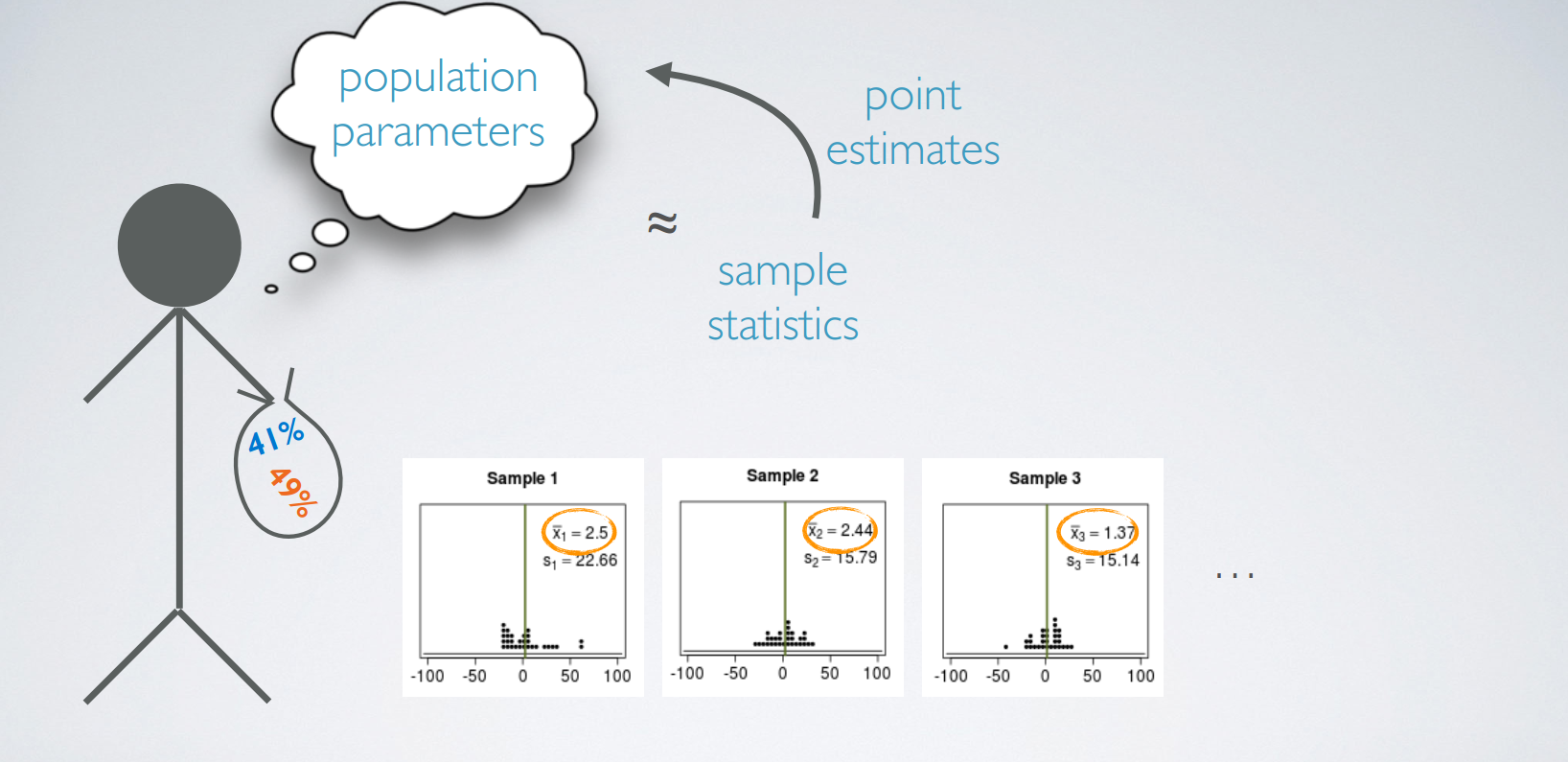
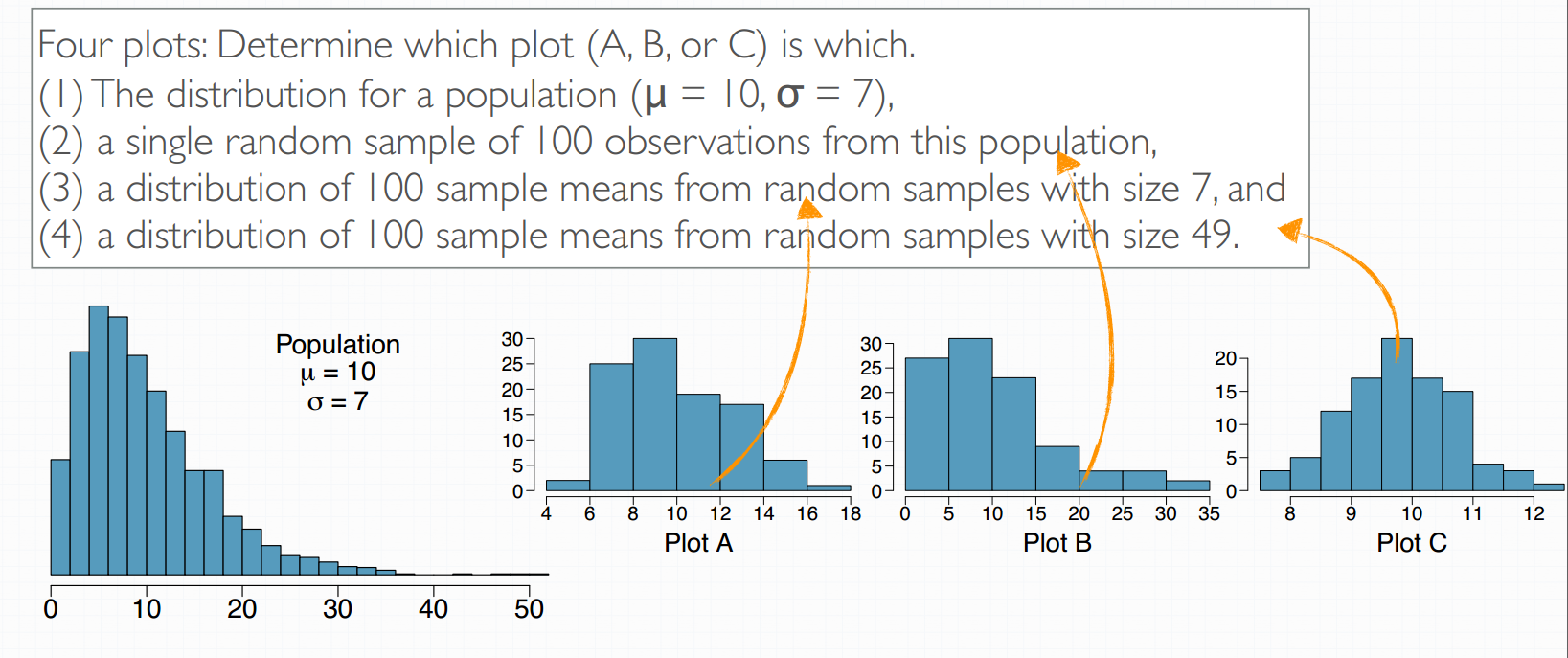
• sample distribution 和sampling distribution

  

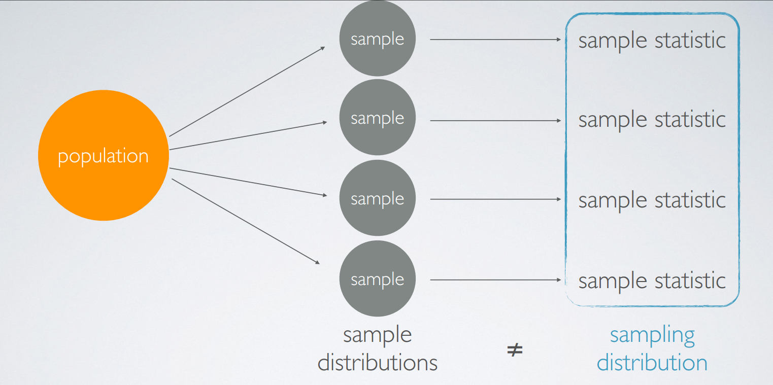
  sample distribution指的是同一样本集之内的分布，sampling distribution指的是多个样本集之间的分布。

  Each one of the samples will have their own distribution, which we call sample distributions. Each observation in these distributions is a randomly sampled unit from the population, say, a person, or a cat, or a dog, depending on what population you're studying.

  The values we recorded from each sample. The sample statistics also now make new distribution. Where each observation is not a unit from the population but a sample statistic. In this case, a sample mean. The distribution of these sample statistics is called the sampling distribution. So the two terms, sample and sampling distributions sound similar, but they're different concepts.

  • example

    

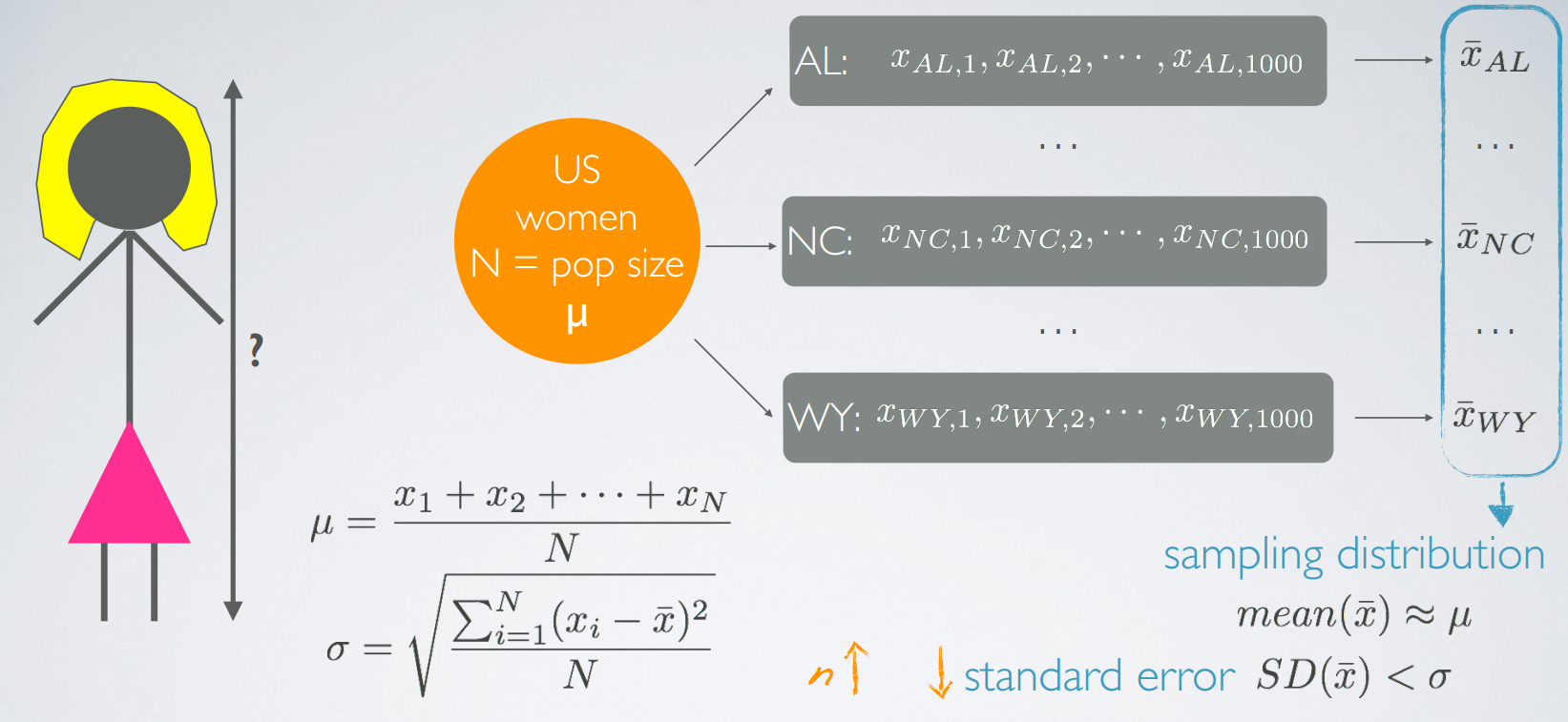
    • standard error指的是不同样本的mean分布的standard deviation

• 中心极限定理

  

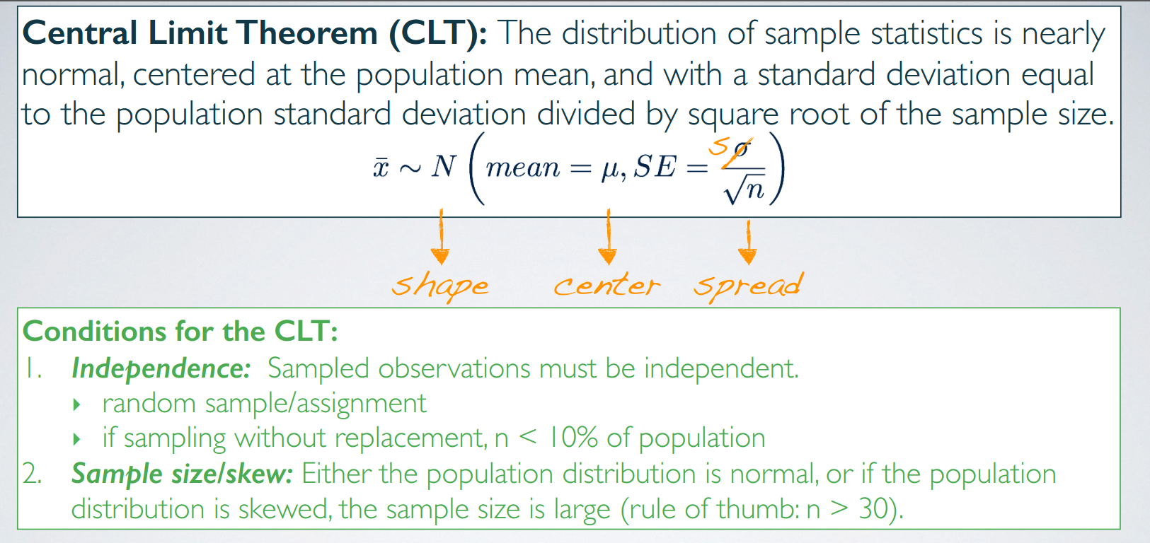
  If sigma is unknown which is often the case, remember sigma is the population standard deviation and oftentimes, we don't have access to the entire population to calculate this number, we use S, the standard sample deviation to estimate the standard error. So that would be the standard deviation of one sample that we happen to have at hand.

  • 关于standard error

    We won't go through a detailed proof of why the standard error is equal to sigma over square root of n, but understanding the inverse relationship between them is very important. As the sample size increases, we would expect samples to yield more consistent sample means, hence the variability among the sample means would be lower, which results in a lower standard error.

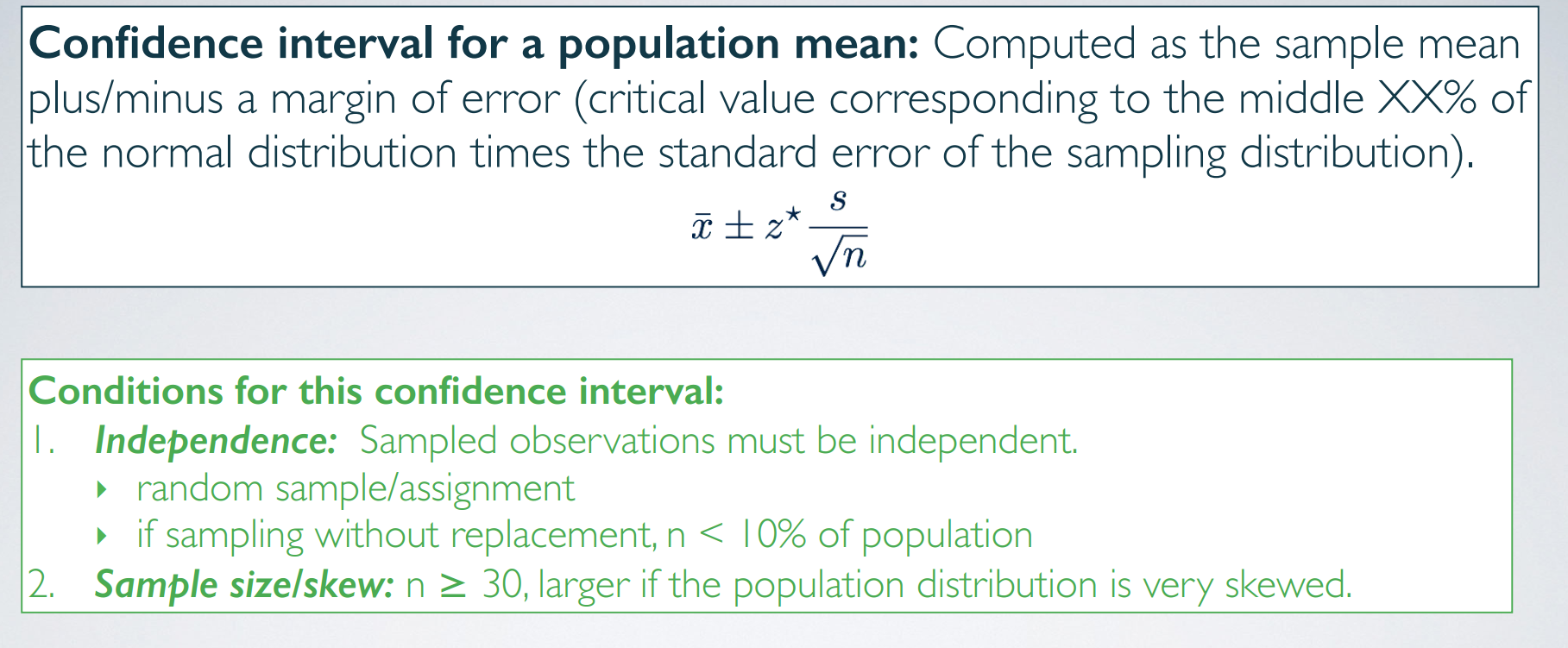
  • 关于两个限制条件

    • independence

      Certain conditions must be met for the central limit theorem to apply. The first on is independence. Samples observations must be independent, and this is very difficult to verify. But it is more likely, if we have used random sampling or assignment depending on whether we have an observational study where we're sampling from the population randomly or we have an experiment where we're randomly assigning experimental units to various treatments. And if sampling without replacement, the sample size N is less than 10% of the population. So we've previously mentioned we love large samples and now we're saying that well, we don't exactly want them to be very large. We're going to talk about why this is the case in a moment.

    • sample size/skew

      The other condition is related to the sample size or skew. Either the population distribution is normal or if the population distribution is skewed or we have no idea what it looks like, the sample size is large. According to the Central Limit Theorem, if the population distribution is normal, the sampling distribution will also be nearly normal, regardless of the sample size. We illustrated this earlier when we working with the outlet where we looked at a sample size of 45 as well as a sample size of 500, and in both instances the sampling distribution was nearly normal. However, if the population distribution is not normal, the more skewed the population distribution, the larger sample size we need for the central limit theorem to apply.

3. example : central limit theorem (for means)

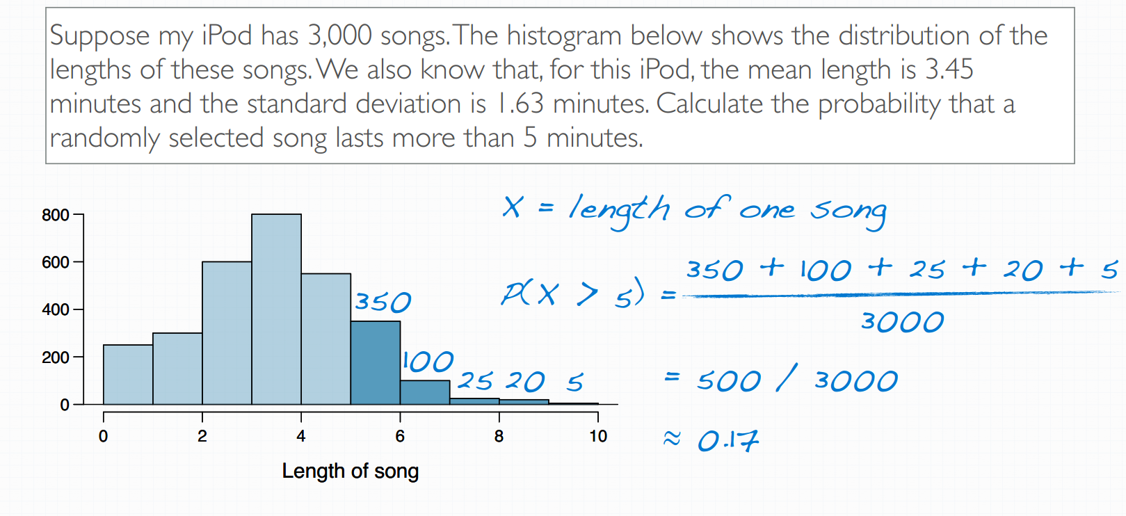
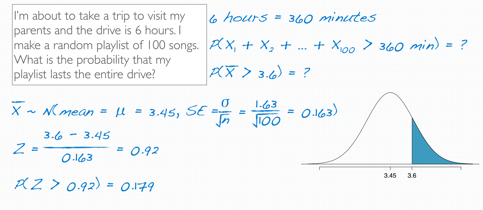
• CLT的应用

  

  • 第一个选项注意3$\sigma$ rule 68%、95%、99.7%

Confidence Interval

1. Confidence Interval(for a mean)

• confidence interval

  

  

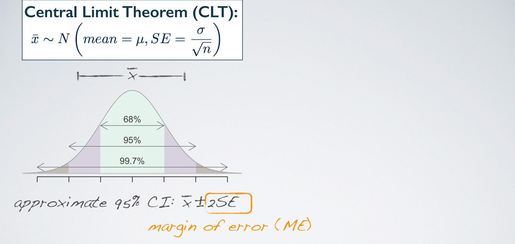
  • margin of error

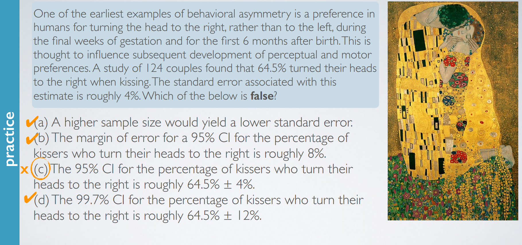
• practice

  

• confidence interval for a population mean

  

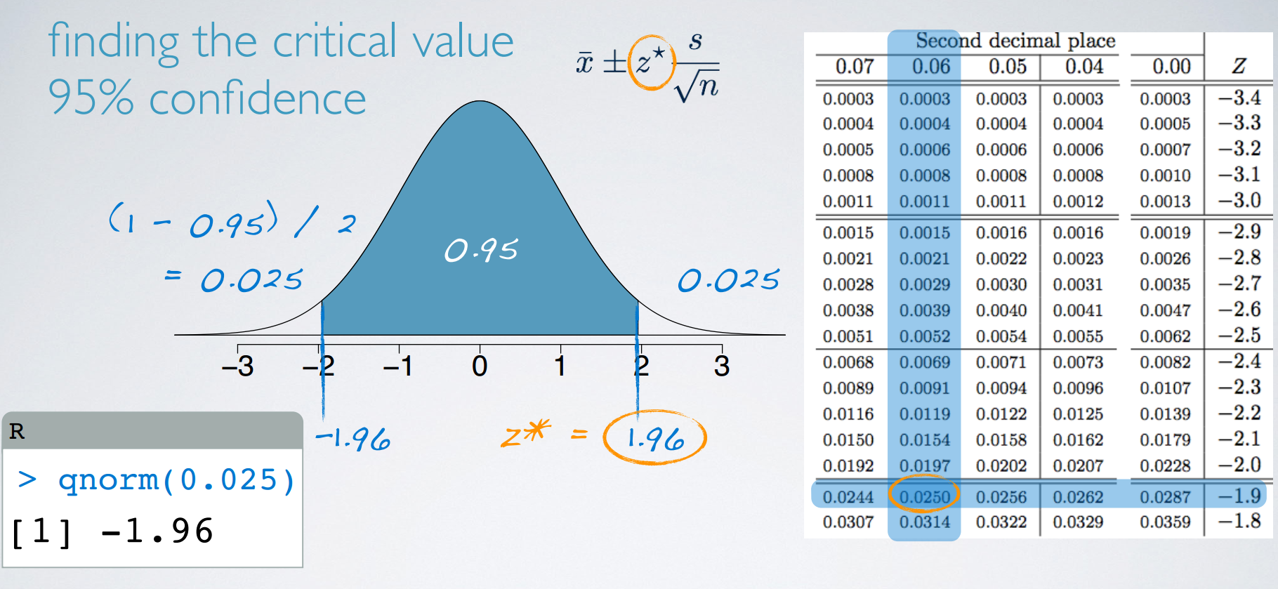
  • finding the critical value 95% confidence
    

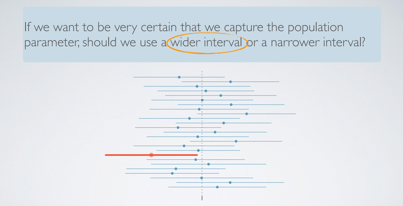
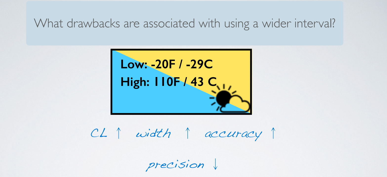
2. Accuracy vs. Precision

We define accuracy in terms of whether or not the confidence interval contains the true population parameter. And precision refers to the width of a confidence interval. So first, we're going to start by defining the confidence level. Then we're going to talk about the interplay between the confidence level and the width of an interval. And then talk about the trade-offs between accuracy and precision.

• confidence level

  

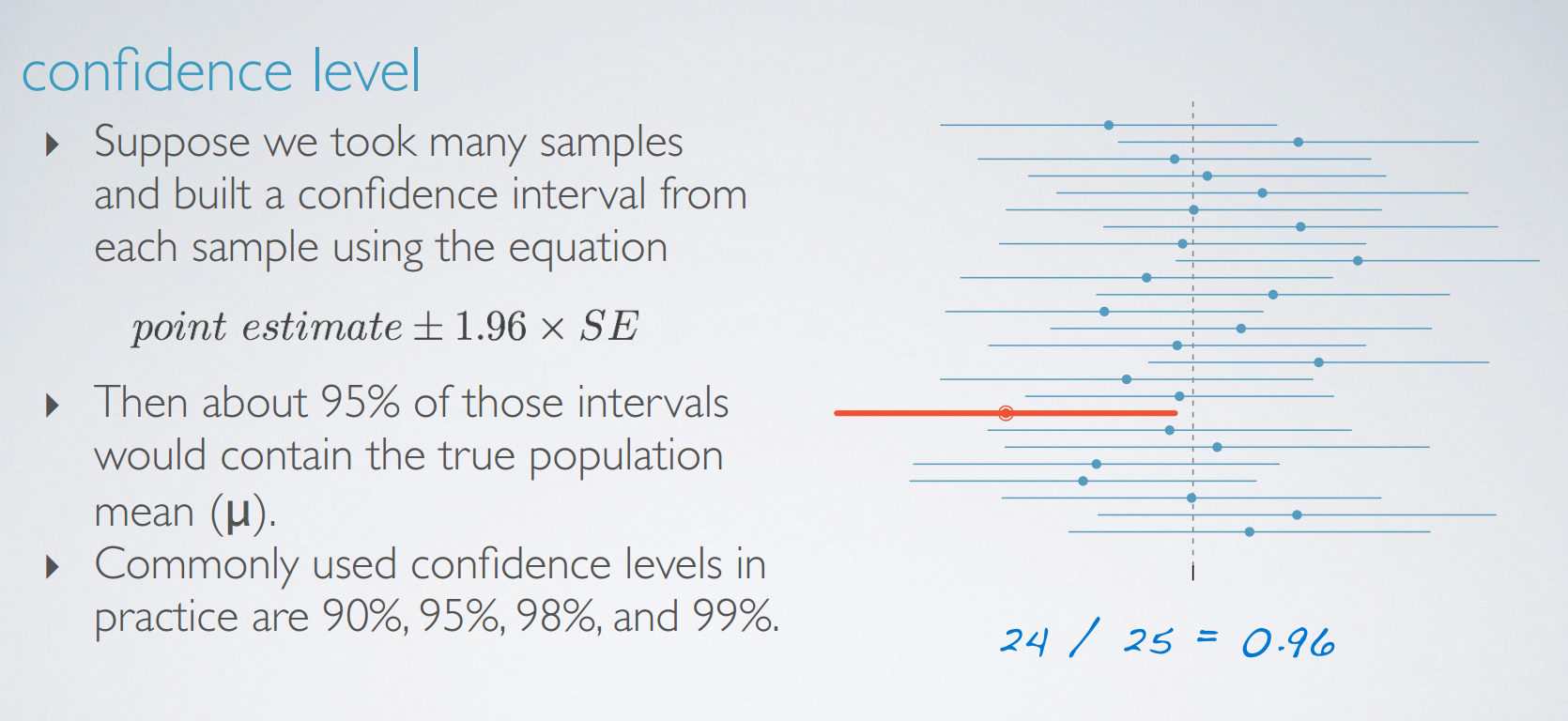
  For example in this figure, the vertical line represents the true population mean, which we rarely know, and each horizontal line is an interval calculated based on a different random sample. There are 25 total intervals plotted, and 24 of them contain the true population mean, and 1 does not. Therefore, the confidence level for these intervals would be 24 over 25, 0.96 or 96%.

  

  

  

• practice

  

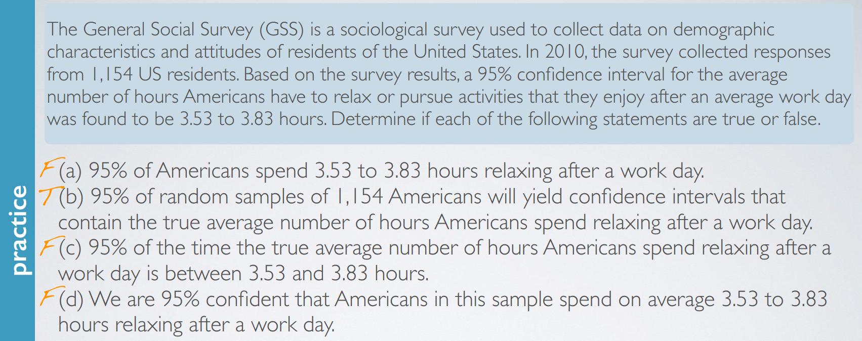
  And lastly, D says we are 95% confident that Americans in this sample spend on average 3.53 to 3.83 hours relaxing after a work day.
  This is not true because remember that the confidence interval is not about the sample mean, but is instead about the population mean. We know exactly what the sample mean is. It has to be between these values because we construct the confidence interval around the sample mean. Therefore, we could actually say that we are 100% confident that Americans in this sample spend on average between 3.53 and 3.83 hours relaxing after an average work day. But that's not a very interesting statement because it's only about the sample, and not about the unknown population parameter that we're after.

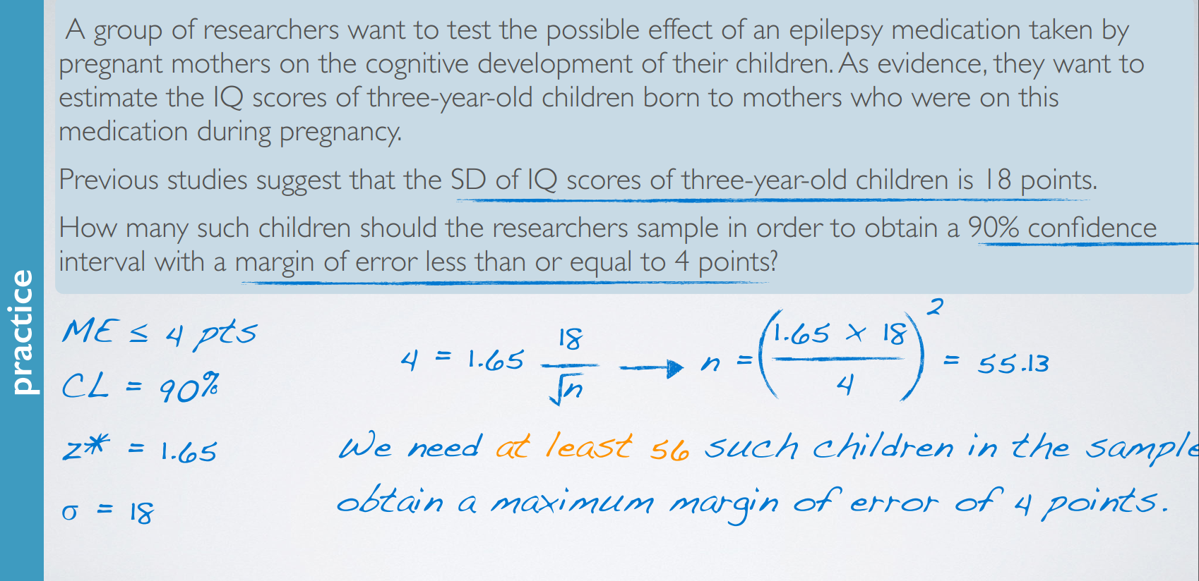
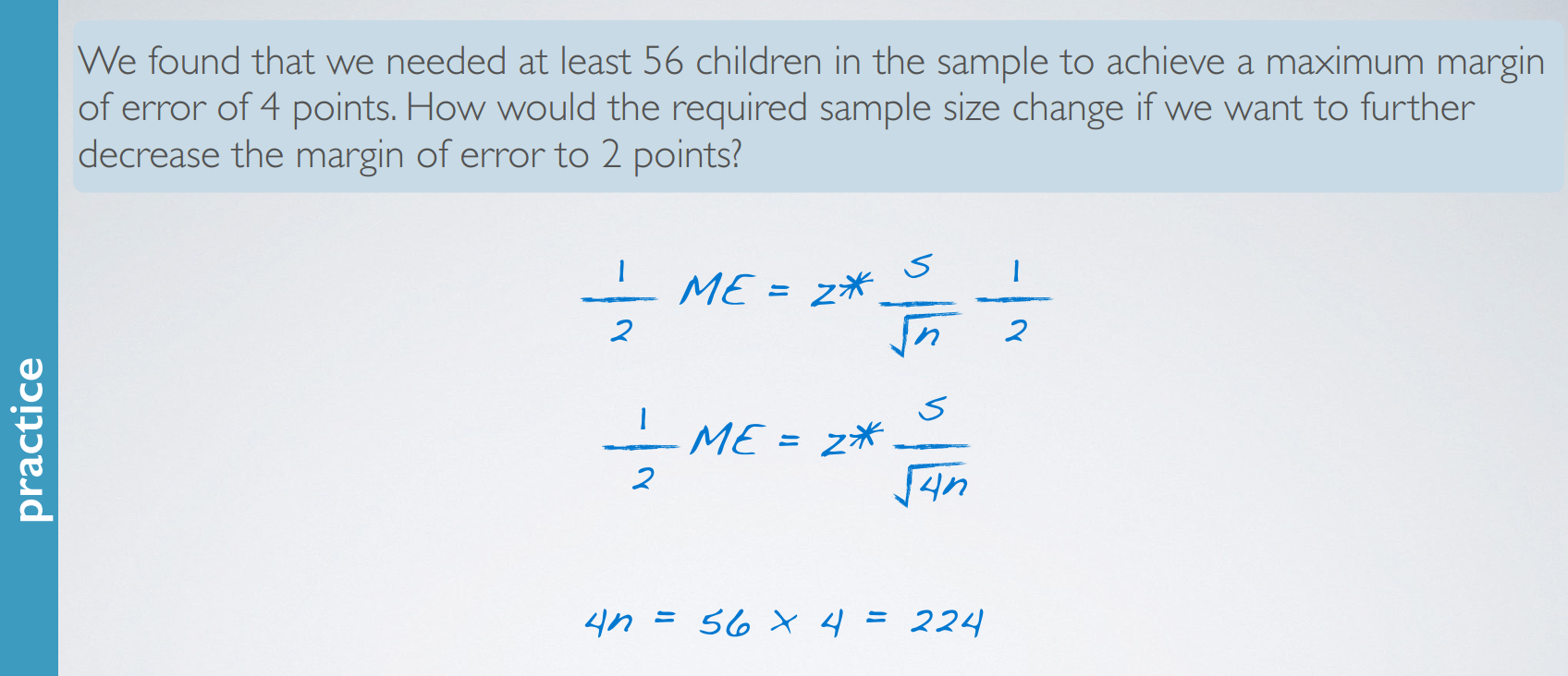
3. required sample size for ME

• backtracking to n for a given ME

  

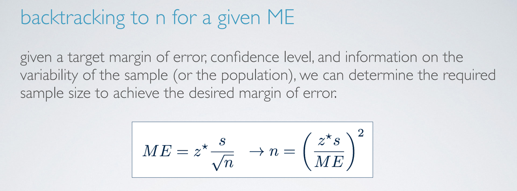
  给定确定的margin error，确定n

• practice

  

  

4. CI examples