《Computer vision》笔记-MobileNet（7）

石文华

1、前言

移动端和其他嵌入式系统通常是内存空间小，能耗要求低的，也就是计算资源有限。一般的模型，比如ImageNet数据集上训练的VGG,googlenet,resnet等，需要巨大的计算资源，所以很难用在嵌入式系统上。MobileNet是一种高效的模型，用于移动和嵌入式视觉应用。

2、深度可分离卷积(depthwise separable convolution)

MobileNet使用技术之一是深度可分离卷积(depthwise separable convolution)代替传统的3D卷积操作，这样可以减少参数数量以及卷积过程中的计算量，但是也会导致特征丢失，使得精度下降。MobileNet其实就是Xception思想的应用。区别就是Xception文章重点在提高精度，而MobileNet重点在压缩模型。
假设输入特征图有M个，大小为DF，输出的特征图是N个，卷积核尺寸是Dk*Dk,那么传统的3D卷积的卷积核是立体的，也就是每一个卷积核都是Dk*Dk*M，总共有N个Dk*Dk*M的卷积核，如下图所示：

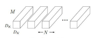
所以总的参数个数为Dk*Dk*M*N,假设输出使用的padding参数是same,则输出特征图大小也是DF，那么总的计算量为Dk*Dk*M*N*DF*DF。
而MobileNet将普通卷积操作分为两部分，第一部分是逐通道卷积，使用M个通道数为1，大小为Dk*Dk的卷积核，每一个卷积核负责其中的一个通道。如下图所示：

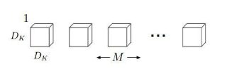
逐通道卷积之后的参数个数为：Dk*Dk*M，同样假设padding为same,则计算量为：Dk*Dk*M*DF*DF
第二部分是点卷积，也就是采用3D的1*1卷积改变通道数，对深度方向上的特征信息进行组合，最终将输出通道数变为指定的数。如下图所示：

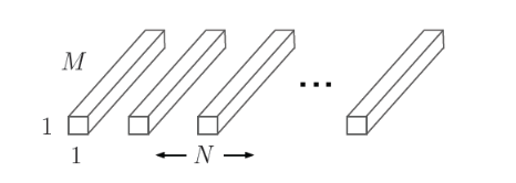
这部分的参数个数为：M*N，padding为same时的计算量为M*N*DF*DF.
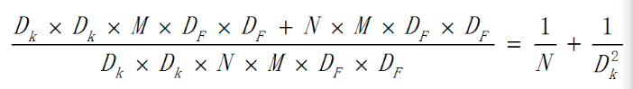
因此这种分离之后的总的计算量为：：Dk*Dk*M*DF*DF+M*N*DF*DF。
深度可分离卷积跟传统3D卷积计算量的比例为：

如下图，左边是3D卷积常见结构，右边是深度可分离卷积的使用方式：

3、宽度因子和分辨率因子

MobileNet有两个简单的全局超参数，分别是宽度因子和分辨率因子，可有效的在延迟和准确率之间做折中。允许我们依据约束条件选择合适大小、低延迟、易满足嵌入式设备要求的模型。
（1）宽度因子
上述的逐通道卷积的卷积核个数通常是M，也就是Dk*Dk*1的卷积核个数等于输入通道数，宽度因子是一个参数为（0，1]之间的参数，作用于通道数，可以理解为按照比例缩减输入通道数。同理，输出的通道数也可以通过这个参数进行按比例缩减。用α表示这个参数，则计算量为：

不同的α取值在ImageNet上的准确率，下图为准确率，参数数量和计算量之间的权衡情况：

（2）分辨率因子
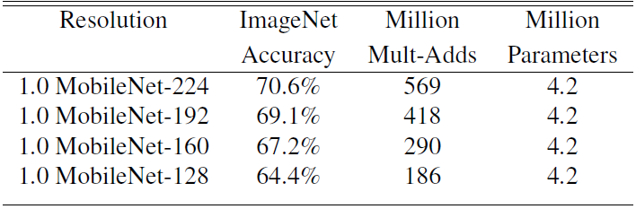
上述的输入特征图大小为DF*DF,分辨率因子取值范围在(0,1]之间，可以理解为对特征图进行下采样，也就是按比例降低特征图的大小，使得输入数据以及由此在每一个模块产生的特征图都变小，用β表示这个参数，结合宽度因子α，则计算量为：

不同的β系数作用于标准MobileNet时，对精度和计算量以的影响（α固定）：

4、改进（MobileNet V2）：

在 MobileNet-V1 基础上结合当下流行的残差思想而设计,V2 主要引入了两个改动：Linear Bottleneck 和 Inverted Residual Blocks。
V1与V2的结构对比：

两者相同的地方在于都采用 Depth-wise (DW) 卷积搭配 Point-wise (PW) 卷积的方式来提特征。
（1）改进一：
V2在 DW 卷积之前新加了一个 PW 卷积，主要目的是为了提升维度数。相比V1直接在每个通道上单独提取特征，V2的这种做法能够先组合不同深度上的特征，并升维，使得特征更加丰富。比直接DW的话，特征提取的效果更好。
（2）改进二：
V2 去掉了第二个 PW 的激活函数。论文作者称其为 Linear Bottleneck。这么做的原因，是因为作者认为激活函数在高维空间能够有效的增加非线性，而在低维空间时则会破坏特征，由Relu的性质，Relu对于负的输入，输出全为零，所以relu会使得一部分特征失效。由于第二个 PW 的主要功能就是降维，再经过Relu的话，又要“损失”一部分特征，因此按照上面的理论，降维之后就不宜再使用 Relu了。如下图所示，一个原始螺旋形被利用随机矩阵T经过ReLU后嵌入到一个n维空间中，然后使用T−1投影到2维空间中。例子中，n=2,3导致信息损失，可以看到流形的中心点之间互相坍塌。同时n=15,30时信息变成高度非凸。

（3）使用短路连接: 倒残差(Inverted Residual)
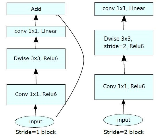
典的残差块是：1x1(压缩)->3x3(卷积)->1x1(升维)，而inverted residual顾名思义是颠倒的残差：1x1(升维)->3x3(dw conv+relu)->1x1(降维+线性变换)，skip-connection(跳过连接)是在低维的瓶颈层间发生的(如下图)，这对于移动端有限的宽带是有益的。连接情况如下图所示(shortcut只在stride==1时才使用)：

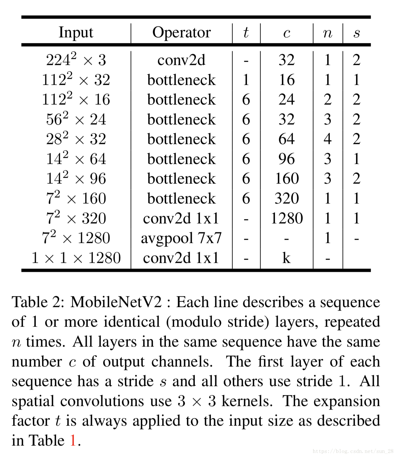
（4）网络结构如下：

由于笔者水平有限，可参考如下github上的代码：https://github.com/tonylins/pytorch-mobilenet-v2/blob/master/MobileNetV2.py

import torch.nn as nn
import math
#传统的3D卷积
def conv_bn(inp, oup, stride):
    return nn.Sequential(
        nn.Conv2d(inp, oup, 3, stride, 1, bias=False),#卷积
        nn.BatchNorm2d(oup),  #bn
        nn.ReLU6(inplace=True)#relu6
    )
#1x1的点卷积
def conv_1x1_bn(inp, oup):
    return nn.Sequential(
        nn.Conv2d(inp, oup, 1, 1, 0, bias=False),
        nn.BatchNorm2d(oup),
        nn.ReLU6(inplace=True)
    )
#倒残差
class InvertedResidual(nn.Module):
    def __init__(self, inp, oup, stride, expand_ratio):#参数分别是输入特征图数，输出特征图数，步长，扩展比例
        super(InvertedResidual, self).__init__()
        self.stride = stride   #步长
        assert stride in [1, 2]   
        hidden_dim = round(inp * expand_ratio)#隐藏层层数，expand_ratio为拓展倍数
        self.use_res_connect = (self.stride == 1 and inp == oup)#是否进跳跃链接
        if expand_ratio == 1:  #不进行扩展
            self.conv = nn.Sequential(
                # dw
                nn.Conv2d(hidden_dim, hidden_dim, 3, stride, 1, groups=hidden_dim, bias=False),#可分离卷积
                nn.BatchNorm2d(hidden_dim),
                nn.ReLU6(inplace=True),
                # pw-linear
                nn.Conv2d(hidden_dim, oup, 1, 1, 0, bias=False),  
                nn.BatchNorm2d(oup),
            )
        else:
            self.conv = nn.Sequential(
                # pw
                nn.Conv2d(inp, hidden_dim, 1, 1, 0, bias=False),
                nn.BatchNorm2d(hidden_dim),
                nn.ReLU6(inplace=True),
                # dw
                nn.Conv2d(hidden_dim, hidden_dim, 3, stride, 1, groups=hidden_dim, bias=False),
                nn.BatchNorm2d(hidden_dim),
                nn.ReLU6(inplace=True),
                # pw-linear
                nn.Conv2d(hidden_dim, oup, 1, 1, 0, bias=False),
                nn.BatchNorm2d(oup),
            )
    def forward(self, x):
        if self.use_res_connect:
            return x + self.conv(x)
        else:
            return self.conv(x)
class MobileNetV2(nn.Module):
    def __init__(self, n_class=1000, input_size=224, width_mult=1.):
        super(MobileNetV2, self).__init__()
        block = InvertedResidual#创建一个倒残差对象
        input_channel = 32   
        last_channel = 1280   
        '''
        t :是输入通道的倍增系数（即中间部分的通道数是输入通道数的多少倍）
        n :是该模块重复次数
        c :是输出通道数
        s :是该模块第一次重复时的 stride（后面重复都是 stride 1）
        '''
        interverted_residual_setting = [
            # t, c, n, s
            [1, 16, 1, 1],
            [6, 24, 2, 2],
            [6, 32, 3, 2],
            [6, 64, 4, 2],
            [6, 96, 3, 1],
            [6, 160, 3, 2],
            [6, 320, 1, 1],
        ]
        # building first layer
        assert input_size % 32 == 0
        input_channel = int(input_channel * width_mult)
        self.last_channel = int(last_channel * width_mult) if width_mult > 1.0 else last_channel
        self.features = [conv_bn(3, input_channel, 2)]
        # building inverted residual blocks
        for t, c, n, s in interverted_residual_setting:
            output_channel = int(c * width_mult)
            for i in range(n):
                if i == 0:
                    self.features.append(block(input_channel, output_channel, s, expand_ratio=t))
                else:
                    self.features.append(block(input_channel, output_channel, 1, expand_ratio=t))
                input_channel = output_channel
        # building last several layers
        self.features.append(conv_1x1_bn(input_channel, self.last_channel))
        # make it nn.Sequential
        self.features = nn.Sequential(*self.features)
        # building classifier
        self.classifier = nn.Sequential(
            nn.Dropout(0.2),
            nn.Linear(self.last_channel, n_class),
        )
        self._initialize_weights()
    def forward(self, x):
        x = self.features(x)
        x = x.mean(3).mean(2)
        x = self.classifier(x)
        return x
    def _initialize_weights(self):
        for m in self.modules():
            if isinstance(m, nn.Conv2d):
                n = m.kernel_size[0] * m.kernel_size[1] * m.out_channels
                m.weight.data.normal_(0, math.sqrt(2. / n))
                if m.bias is not None:
                    m.bias.data.zero_()
            elif isinstance(m, nn.BatchNorm2d):
                m.weight.data.fill_(1)
                m.bias.data.zero_()
            elif isinstance(m, nn.Linear):
                n = m.weight.size(1)
                m.weight.data.normal_(0, 0.01)
                m.bias.data.zero_()
model= MobileNetV2()
print(model)    

参考文献：
https://blog.csdn.net/t800ghb/article/details/78879612
https://www.cnblogs.com/CodingML-1122/p/9043078.html
https://blog.csdn.net/u011995719/article/details/79135818
https://zhuanlan.zhihu.com/p/33075914
https://zhuanlan.zhihu.com/p/39386719
https://mp.weixin.qq.com/s/T6S1_cFXPEuhRAkJo2m8Ig
https://blog.csdn.net/qq_31531635/article/details/80550412
https://github.com/tonylins/pytorch-mobilenet-v2/blob/master/MobileNetV2.py