@spiritnotes
2016-03-07T14:27:27.000000Z
字数 8272
阅读 6590
机器学习实践 -- digits数据集
机器学习实践
获取
from sklearn import datasetsdigits = datasets.load_digits()
其包含的是手写体的数字,从0到9。数据集总共有1797个样本,每个样本由64个特征组成,分别为其手写体对应的8×8像素表示,每个特征取值0~16。
In [20]:data.shape, target.shape, data.min(), data.max()Out[20]:((1797, 64), (1797,), 0.0, 16.0)
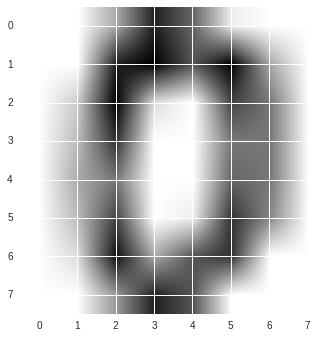
该数据还提供了images表示,其与data中数据一致,只是转变为了8*8的二维数组表示。针对单个图像表示,可见图如下:
plt.imshow(images[0], cmap='binary')
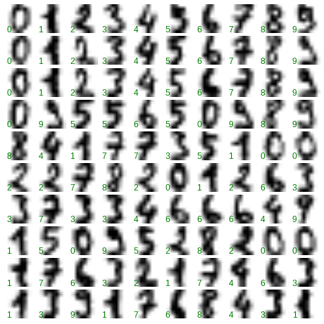
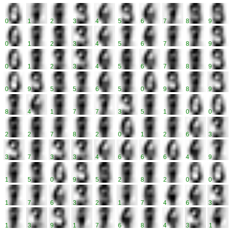
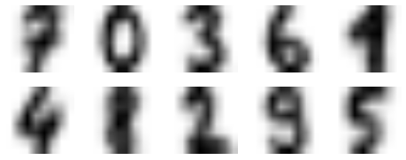
针对前100个样本,描述图像如下:
fig, axes = plt.subplots(10, 10, figsize=(8, 8))fig.subplots_adjust(hspace=0.1, wspace=0.1)for i, ax in enumerate(axes.flat):ax.imshow(images[i], cmap='binary')ax.text(0.05, 0.05, str(target[i]), transform=ax.transAxes, color='green')ax.set_xticks([]) #清除坐标ax.set_yticks([])
分析
该问题是一个典型的分类问题。数据集有64个特征,而且特征仅表示像素位置上的强度值,没有特殊的物理意义,因此无法直接在64个维度上进行分析。可以先降维进行分析。
PCA降维
from sklearn.decomposition import PCApca = PCA(n_components=2)data_pca = pca.fit_transform(data)plt.scatter(data_pca[:, 0], data_pca[:, 1], c=target, edgecolor='none', alpha=0.5, cmap=plt.cm.get_cmap('nipy_spectral', 10))plt.colorbar();
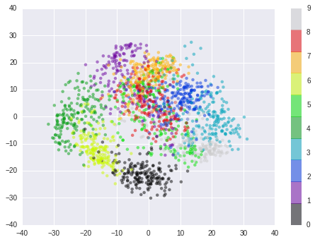
从图中我们可以看到降维后大部分点比较聚集,能够区分的。部分点有交叉是由于其降维后导致的特征丢失,例如针对图中的(-10,-20)还原如图,位于0和6的交界处。
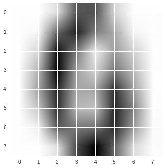
data_ = pca.inverse_transform(array([[-10,-20]]))plt.imshow(data_[0].reshape((8,8)), cmap='binary')
对前100个图像进行降维还原如下图:
data_repca = pca.inverse_transform(data_pca)images_repca = data_repca.copy()images_repca.shape = (1797, 8, 8)
可见其缺失丢失了较多特征。PCA降维的能量占比曲线如下,其2维能量占比为28.5%,还原度很低
sb.set()pca_ = PCA().fit(data)plt.plot(np.cumsum(pca_.explained_variance_ratio_))plt.xlabel('number of components')plt.ylabel('cumulative explained variance');
IsoMap
from sklearn.manifold import Isomapiso = Isomap(n_components=2)data_projected = iso.fit_transform(data)plt.scatter(data_projected[:, 0], data_projected[:, 1], c=target,edgecolor='none', alpha=0.5, cmap=plt.cm.get_cmap('nipy_spectral', 10));plt.colorbar(label='digit label', ticks=range(10))plt.clim(-0.5, 9.5)
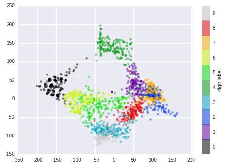
从IsoMap图上可见不同的数字区分得更开,而易混淆的地方也正是近似的地方,如2和7、3和9。
模型选择
从数据上看线性分类即可解决该问题,我们可选的模型有KNN,逻辑回归,SVM,决策树,随机森林等。
KNN
from sklearn.neighbors import KNeighborsClassifierfrom sklearn.grid_search import GridSearchCVclf = KNeighborsClassifier()n_neighbors = [1,2,3,5,8,10,15,20,25,30,35,40]weights = ['uniform','distance']param_grid = [{'n_neighbors': n_neighbors, 'weights': weights}]grid_search = GridSearchCV(clf, param_grid=param_grid, cv=10)grid_search.fit(data, target)
其结果如下
In [56]:grid_search.best_score_, grid_search.best_estimator_, grid_search.best_params_,Out[56]:(0.97829716193656091,KNeighborsClassifier(algorithm='auto', leaf_size=30, metric='minkowski',metric_params=None, n_jobs=1, n_neighbors=3, p=2,weights='distance'),{'n_neighbors': 3, 'weights': 'distance'})
逻辑回归
from sklearn.grid_search import GridSearchCVfrom sklearn.linear_model import LogisticRegressionclf = LogisticRegression(penalty='l2')C = [0.1, 0.5, 1, 5, 10]param_grid = [{'C': C}]grid_search = GridSearchCV(clf, param_grid=param_grid, cv=10)grid_search.fit(data, target)
执行结果:
In [63]:grid_search.best_score_, grid_search.best_estimator_,grid_search.best_params_Out[63]:(0.9360044518642181,LogisticRegression(C=0.1, class_weight=None, dual=False, fit_intercept=True,intercept_scaling=1, max_iter=100, multi_class='ovr', n_jobs=1,penalty='l2', random_state=None, solver='liblinear', tol=0.0001,verbose=0, warm_start=False),{'C': 0.1})
SVM
from sklearn.grid_search import GridSearchCVfrom sklearn.svm import SVCclf = SVC()C = [0.1, 0.5, 1, 5, 10]kernel = ['linear', 'poly', 'rbf']param_grid = [{'C': C, 'kernel':kernel}]grid_search = GridSearchCV(clf, param_grid=param_grid, cv=10)grid_search.fit(data, target)
结果如下:
In [73]:grid_search.best_score_, grid_search.best_estimator_, grid_search.best_params_Out[73]:(0.97885364496382865, SVC(C=0.1, cache_size=200, class_weight=None, coef0=0.0,decision_function_shape=None, degree=3, gamma='auto', kernel='poly',max_iter=-1, probability=False, random_state=None, shrinking=True,tol=0.001, verbose=False), {'C': 0.1, 'kernel': 'poly'})In [74]:grid_search.grid_scores_Out[74]:[mean: 0.96105, std: 0.02191, params: {'kernel': 'linear', 'C': 0.1},mean: 0.97885, std: 0.01931, params: {'kernel': 'poly', 'C': 0.1},mean: 0.10184, std: 0.00153, params: {'kernel': 'rbf', 'C': 0.1},mean: 0.96105, std: 0.02191, params: {'kernel': 'linear', 'C': 0.5},mean: 0.97885, std: 0.01931, params: {'kernel': 'poly', 'C': 0.5},mean: 0.11130, std: 0.00709, params: {'kernel': 'rbf', 'C': 0.5},mean: 0.96105, std: 0.02191, params: {'kernel': 'linear', 'C': 1},mean: 0.97885, std: 0.01931, params: {'kernel': 'poly', 'C': 1},mean: 0.48692, std: 0.06936, params: {'kernel': 'rbf', 'C': 1},mean: 0.96105, std: 0.02191, params: {'kernel': 'linear', 'C': 5},mean: 0.97885, std: 0.01931, params: {'kernel': 'poly', 'C': 5},mean: 0.52031, std: 0.06315, params: {'kernel': 'rbf', 'C': 5},mean: 0.96105, std: 0.02191, params: {'kernel': 'linear', 'C': 10},mean: 0.97885, std: 0.01931, params: {'kernel': 'poly', 'C': 10},mean: 0.52031, std: 0.06315, params: {'kernel': 'rbf', 'C': 10}]
决策树
from sklearn.grid_search import GridSearchCVfrom sklearn.tree import DecisionTreeClassifierclf = DecisionTreeClassifier()criterion = ['gini','entropy']max_depth = [10, 15, 20, 30, None]min_samples_split = [2, 3, 5, 8, 10]min_samples_leaf = [1, 2, 3, 5, 8]param_grid = [{'criterion': criterion, 'max_depth':max_depth, 'min_samples_split':min_samples_split, 'min_samples_leaf':min_samples_leaf}]grid_search = GridSearchCV(clf, param_grid=param_grid, cv=10)grid_search.fit(data, target)
结果如下:
(0.83750695603784087,DecisionTreeClassifier(class_weight=None, criterion='entropy', max_depth=10,max_features=None, max_leaf_nodes=None, min_samples_leaf=1,min_samples_split=2, min_weight_fraction_leaf=0.0,presort=False, random_state=None, splitter='best'),{'criterion': 'entropy','max_depth': 10,'min_samples_leaf': 1,'min_samples_split': 2})
随机森林
from sklearn.grid_search import GridSearchCVfrom sklearn.ensemble import RandomForestClassifierclf = RandomForestClassifier(random_state=0)n_estimators = [10, 20, 35, 50, 80, 100, 120, 150, 200]param_grid = [{'n_estimators': n_estimators}]grid_search = GridSearchCV(clf, param_grid=param_grid, cv=10)grid_search.fit(data, target)
结果为:
(0.95325542570951582,RandomForestClassifier(bootstrap=True, class_weight=None, criterion='gini',max_depth=None, max_features='auto', max_leaf_nodes=None,min_samples_leaf=1, min_samples_split=2,min_weight_fraction_leaf=0.0, n_estimators=120, n_jobs=1,oob_score=False, random_state=0, verbose=0, warm_start=False),{'n_estimators': 120})
汇总
| Classifier | score | std |
|---|---|---|
| KNN | 0.978 | 0.016 |
| LogisticRegression | 0.936 | 0.032 |
| SVC | 0.979 | 0.019 |
| DecisionTreeClassifier | 0.837 | |
| RandomForestClassifier | 0.953 | 0.019 |
结果分析
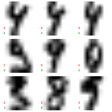
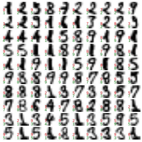
以SVC为例分析看下分错的样本形态。
svc_ = SVC(C=0.1, cache_size=200, class_weight=None, coef0=0.0,decision_function_shape=None, degree=3, gamma='auto', kernel='poly',max_iter=-1, probability=False, random_state=None, shrinking=True,tol=0.001, verbose=False)from sklearn.cross_validation import train_test_splitXtrain, Xtest, ytrain, ytest = train_test_split(data, target, test_size=0.2,random_state=2)svc_.fit(Xtrain, ytrain)svc_.score(Xtest, ytest) ## 0.97499999999999998
查看混淆矩阵
from sklearn.metrics import confusion_matrixprint(confusion_matrix(ytest, svc_.predict(Xtest)))[[31 0 0 0 1 0 0 0 0 0][ 0 44 0 0 0 0 0 0 0 0][ 0 0 31 0 0 0 0 0 0 0][ 0 0 0 35 0 0 0 0 1 0][ 0 0 0 0 32 0 0 0 3 0][ 0 0 0 0 0 42 0 0 0 1][ 0 0 0 0 0 0 35 0 0 0][ 0 0 0 0 0 0 0 40 0 0][ 0 0 0 0 0 0 0 0 35 1][ 0 0 0 0 0 1 0 0 1 26]]
打印判断错误的数字:
Ypre = svc_.predict(Xtest)Xerror, Yerror, Ypreerror = Xtest[Ypre!=ytest], ytest[Ypre!=ytest], Ypre[Ypre!=ytest]Xerror_images = Xerror.reshape((len(Xerror), 8, 8))fig, axes = plt.subplots(3, 3, figsize=(8, 8))fig.subplots_adjust(hspace=0.1, wspace=0.1)for i, ax in enumerate(axes.flat):ax.imshow(Xerror_images[i], cmap='binary')ax.text(0.05, 0.05, str(Yerror[i]), transform=ax.transAxes, color='green')ax.text(0.05, 0.2, str(Ypreerror[i]), transform=ax.transAxes, color='red')ax.set_xticks([]) #清除坐标ax.set_yticks([])
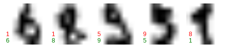
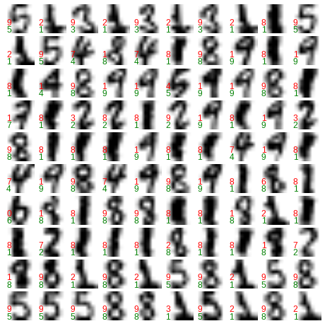
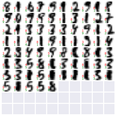
而另外一种随机测试集划分其结果如下。
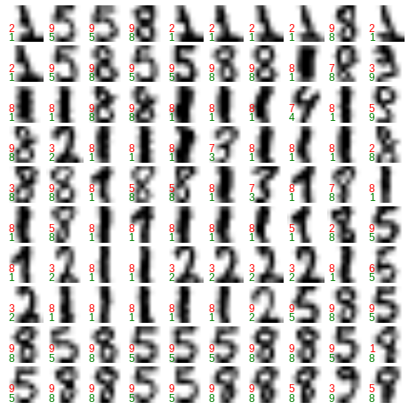
聚类 K-Means
针对该数据集我们可以进行聚类,无监督学习。
from sklearn.cluster import KMeansest = KMeans(n_clusters=10)pres = est.fit_predict(data)
可以通过查看质心来确认当前的分类结果
fig = plt.figure(figsize=(8, 3))for i in range(10):ax = fig.add_subplot(2, 5, 1 + i, xticks=[], yticks=[])ax.imshow(est.cluster_centers_[i].reshape((8, 8)), cmap=plt.cm.binary)
trans = [7,0,3,6,1,4,8,2,9,5]error_indexs = np.zeros(len(data))for i in range(len(error_indexs)):if target[i] != trans[est.labels_[i]]:error_indexs[i] = 1error_indexs = error_indexs != 0Xerror, Yerror, Ypreerror = data[error_indexs], target[error_indexs], est.labels_[error_indexs]
错误了375个,错误率约为20.8%。对于非监督学习来说,准确率能有80%,很不错了。查看一下错误的聚类如下
fig, axes = plt.subplots(10, 10, figsize=(8, 8))fig.subplots_adjust(hspace=0.1, wspace=0.1)for i, ax in enumerate(axes.flat):ax.imshow(Xerror[i].reshape(8,8), cmap='binary')ax.text(0.05, 0.05, str(Yerror[i]), transform=ax.transAxes, color='green')ax.text(0.05, 0.3, str(trans[Ypreerror[i]]), transform=ax.transAxes, color='red')ax.set_xticks([]) #清除坐标ax.set_yticks([])
code
github: https://github.com/spiritwiki/codes/tree/master/data_digits
