PyCon 2015 Scikit-learn Tutorial by Jake VanderPlas

sklearn

An Introduction to scikit-learn: Machine Learning in Python

Instructor: Jake VanderPlas
- email: jakevdp@uw.edu
- twitter: @jakevdp
- github: jakevdp

01-Preliminaries

确认软件是否已经正常安装

02.1-Machine-Learning-Intro

What is Machine Learning?

SGD分类

from sklearn.datasets.samples_generator import make_blobs
from sklearn.linear_model import SGDClassifier
clf = SGDClassifier(loss="hinge", alpha=0.01, n_iter=200, fit_intercept=True)

Representation of Data in Scikit-learn

Most machine learning algorithms implemented in scikit-learn expect data to be stored in a two-dimensional array or matrix. The arrays can be either numpy arrays, or in some cases scipy.sparse matrices. The size of the array is expected to be [n_samples, n_features]
n_samples: The number of samples: each sample is an item to process (e.g. classify). A sample can be a document, a picture, a sound, a video, an astronomical object, a row in database or CSV file, or whatever you can describe with a fixed set of quantitative traits.
n_features: The number of features or distinct traits that can be used to describe each item in a quantitative manner. Features are generally real-valued, but may be boolean or discrete-valued in some cases.

A Simple Example: the Iris Dataset

from sklearn.datasets import load_iris
iris = load_iris()

可视化

import numpy as np
import matplotlib.pyplot as plt
x_index = 0
y_index = 1
# this formatter will label the colorbar with the correct target names
formatter = plt.FuncFormatter(lambda i, *args: iris.target_names[int(i)])
plt.scatter(iris.data[:, x_index], iris.data[:, y_index],
            c=iris.target, cmap=plt.cm.get_cmap('RdYlBu', 3))
plt.colorbar(ticks=[0, 1, 2], format=formatter)
plt.clim(-0.5, 2.5)
plt.xlabel(iris.feature_names[x_index])
plt.ylabel(iris.feature_names[y_index]);

Other Available Data

• Packaged Data: these small datasets are packaged with the scikit-learn installation, and can be downloaded using the tools in sklearn.datasets.load_*
• Downloadable Data: these larger datasets are available for download, and scikit-learn includes tools which streamline this process. These tools can be found in sklearn.datasets.fetch_*
• Generated Data: there are several datasets which are generated from models based on a random seed. These are available in the sklearn.datasets.make_*

02.2-Basic-Principles

The Scikit-learn Estimator Object

Estimator

from sklearn.linear_model import LinearRegression

Estimator parameters

All the parameters of an estimator can be set when it is instantiated, and have suitable default values
print(model);print(model.normalize)

fit

model.residues_

Supervised Learning: Classification and Regression

knn = neighbors.KNeighborsClassifier(n_neighbors=5)
X_fit = np.linspace(0, 1, 100)[:, np.newaxis]
y_fit = model.predict(X_fit)
from sklearn.ensemble import RandomForestRegressor
model = RandomForestRegressor()

Unsupervised Learning: Dimensionality Reduction and Clustering

from sklearn.decomposition import PCA
pca = PCA(n_components=2)
pca.fit(X)
X_reduced = pca.transform(X)
pl.scatter(X_reduced[:, 0], X_reduced[:, 1], c=y, cmap='RdYlBu')
for component in pca.components_:
    print(" + ".join("%.3f x %s" % (value, name)
                     for value, name in zip(component,
                                            iris.feature_names)))

from sklearn.cluster import KMeans
k_means = KMeans(n_clusters=3, random_state=0) # Fixing the RNG in kmeans
k_means.fit(X)
y_pred = k_means.predict(X)
pl.scatter(X_reduced[:, 0], X_reduced[:, 1], c=y_pred,
           cmap='RdYlBu');

Recap: Scikit-learn's estimator interface

Scikit-learn strives to have a uniform interface across all methods, and we'll see examples of these below. Given a scikit-learn estimator object named model, the following methods are available:

• Available in all Estimators
  
  • model.fit() : fit training data. For supervised learning applications, this accepts two arguments: the data X and the labels y (e.g. model.fit(X, y)). For unsupervised learning applications, this accepts only a single argument, the data X (e.g. model.fit(X)).
• Available in supervised estimators
  
  • model.predict() : given a trained model, predict the label of a new set of data. This method accepts one argument, the new data X_new (e.g. model.predict(X_new)), and returns the learned label for each object in the array.
  • model.predict_proba() : For classification problems, some estimators also provide this method, which returns the probability that a new observation has each categorical label. In this case, the label with the highest probability is returned by model.predict().
  • model.score() : for classification or regression problems, most (all?) estimators implement a score method. Scores are between 0 and 1, with a larger score indicating a better fit.
• Available in unsupervised estimators
  
  • model.predict() : predict labels in clustering algorithms.
  • model.transform() : given an unsupervised model, transform new data into the new basis. This also accepts one argument X_new, and returns the new representation of the data based on the unsupervised model.
  • model.fit_transform() : some estimators implement this method, which more efficiently performs a fit and a transform on the same input data.

Model Validation

从训练数据到泛化到未知数据

#混淆矩阵
from sklearn.metrics import confusion_matrix
print(confusion_matrix(y, y_pred))
#训练测试数据集划分
from sklearn.cross_validation import train_test_split
Xtrain, Xtest, ytrain, ytest = train_test_split(X, y)

Quick Application: Optical Character Recognition

#加载数据
from sklearn import datasets
digits = datasets.load_digits()
#可视化
fig, axes = plt.subplots(10, 10, figsize=(8, 8))
fig.subplots_adjust(hspace=0.1, wspace=0.1)
for i, ax in enumerate(axes.flat):
    ax.imshow(digits.images[i], cmap='binary')
    ax.text(0.05, 0.05, str(digits.target[i]),
            transform=ax.transAxes, color='green')
    ax.set_xticks([])
    ax.set_yticks([])

Unsupervised Learning: Dimensionality Reduction

from sklearn.manifold import Isomap
plt.scatter(data_projected[:, 0], data_projected[:, 1], c=digits.target,
            edgecolor='none', alpha=0.5, cmap=plt.cm.get_cmap('nipy_spectral', 10));
plt.colorbar(label='digit label', ticks=range(10))
plt.clim(-0.5, 9.5)

Classification on Digits

使用逻辑回归

03.1-Classification-SVMs

Support Vector Machines: Maximizing the Margin

from sklearn.svm import SVC # "Support Vector Classifier"
clf = SVC(kernel='linear')
clf.fit(X, y)
clf = SVC(kernel='rbf')
clf.fit(X, y)

03.2-Regression-Forests

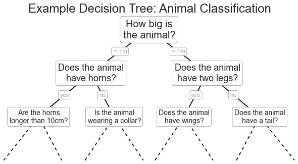
Motivating Random Forests: Decision Trees

# 产生数据
from sklearn.datasets import make_blobs
X, y = make_blobs(n_samples=300, centers=4,
                  random_state=0, cluster_std=1.0)
plt.scatter(X[:, 0], X[:, 1], c=y, s=50, cmap='rainbow');

Decision Trees and over-fitting

Ensembles of Estimators: Random Forests

04.1-Dimensionality-PCA

Dimensionality Reduction: Principal Component Analysis in-depth

#产生数据
np.random.seed(1)
X = np.dot(np.random.random(size=(2, 2)), np.random.normal(size=(2, 200))).T
plt.plot(X[:, 0], X[:, 1], 'o')
plt.axis('equal');
#训练
from sklearn.decomposition import PCA
pca = PCA(n_components=2)
pca.fit(X)
print(pca.explained_variance_)
print(pca.components_)
#可视化
plt.plot(X[:, 0], X[:, 1], 'o', alpha=0.5)
for length, vector in zip(pca.explained_variance_, pca.components_):
    v = vector * 3 * np.sqrt(length)
    plt.plot([0, v[0]], [0, v[1]], '-k', lw=3)
plt.axis('equal');
#
clf = PCA(0.95) # keep 95% of variance
X_trans = clf.fit_transform(X)
print(X.shape)
print(X_trans.shape)
X_new = clf.inverse_transform(X_trans)
plt.plot(X[:, 0], X[:, 1], 'o', alpha=0.2)
plt.plot(X_new[:, 0], X_new[:, 1], 'ob', alpha=0.8)
plt.axis('equal');

04.2-Clustering-KMeans

# 产生数据
from sklearn.datasets.samples_generator import make_blobs
X, y = make_blobs(n_samples=300, centers=4,
                  random_state=0, cluster_std=0.60)
plt.scatter(X[:, 0], X[:, 1], s=50);
# 聚类
from sklearn.cluster import KMeans
est = KMeans(4)  # 4 clusters
est.fit(X)
y_kmeans = est.predict(X)
plt.scatter(X[:, 0], X[:, 1], c=y_kmeans, s=50, cmap='rainbow');
# 可视化
from fig_code import plot_kmeans_interactive
plot_kmeans_interactive();

Example: KMeans for Color Compression

# reduce the size of the image for speed
image = china[::3, ::3]
n_colors = 64
X = (image / 255.0).reshape(-1, 3)
model = KMeans(n_colors)
labels = model.fit_predict(X)
colors = model.cluster_centers_
new_image = colors[labels].reshape(image.shape)
new_image = (255 * new_image).astype(np.uint8)
# create and plot the new image
with sns.axes_style('white'):
    plt.figure()
    plt.imshow(image)
    plt.title('input')
    plt.figure()
    plt.imshow(new_image)
    plt.title('{0} colors'.format(n_colors))

04.3-Density-GMM

Here we'll explore Gaussian Mixture Models, which is an unsupervised clustering & density estimation technique.

np.random.seed(2)
x = np.concatenate([np.random.normal(0, 2, 2000),
                    np.random.normal(5, 5, 2000),
                    np.random.normal(3, 0.5, 600)])
plt.hist(x, 80, normed=True)
plt.xlim(-10, 20);
from sklearn.mixture import GMM
clf = GMM(4, n_iter=500, random_state=3).fit(x)
xpdf = np.linspace(-10, 20, 1000)
density = np.exp(clf.score(xpdf))
plt.hist(x, 80, normed=True, alpha=0.5)
plt.plot(xpdf, density, '-r')
plt.xlim(-10, 20);
# Note that this density is fit using a mixture of Gaussians, which we can examine by looking at the means_, covars_, and weights_ attributes:
clf.means_
clf.covars_
clf.weights_
plt.hist(x, 80, normed=True, alpha=0.3)
plt.plot(xpdf, density, '-r')
for i in range(clf.n_components):
    pdf = clf.weights_[i] * stats.norm(clf.means_[i, 0],
                                       np.sqrt(clf.covars_[i, 0])).pdf(xpdf)
    plt.fill(xpdf, pdf, facecolor='gray',
             edgecolor='none', alpha=0.3)
plt.xlim(-10, 20);

How many Gaussians?

Given a model, we can use one of several means to evaluate how well it fits the data. For example, there is the Aikaki Information Criterion (AIC) and the Bayesian Information Criterion (BIC)

print(clf.bic(x))
print(clf.aic(x))
n_estimators = np.arange(1, 10)
clfs = [GMM(n, n_iter=1000).fit(x) for n in n_estimators]
bics = [clf.bic(x) for clf in clfs]
aics = [clf.aic(x) for clf in clfs]
plt.plot(n_estimators, bics, label='BIC')
plt.plot(n_estimators, aics, label='AIC')
plt.legend();

Example: GMM For Outlier Detection

GMM is what's known as a Generative Model: it's a probabilistic model from which a dataset can be generated.
One thing that generative models can be useful for is outlier detection: we can simply evaluate the likelihood of each point under the generative model; the points with a suitably low likelihood (where "suitable" is up to your own bias/variance preference) can be labeld outliers.

log_likelihood = clf.score_samples(y)[0]
plt.plot(y, log_likelihood, '.k');
detected_outliers = np.where(log_likelihood < -9)[0]
print("true outliers:")
print(true_outliers)
print("\ndetected outliers:")
print(detected_outliers)
set(true_outliers) - set(detected_outliers)

Other Density Estimators

from sklearn.neighbors import KernelDensity
kde = KernelDensity(0.15).fit(x[:, None])
density_kde = np.exp(kde.score_samples(xpdf[:, None]))
plt.hist(x, 80, normed=True, alpha=0.5)
plt.plot(xpdf, density, '-b', label='GMM')
plt.plot(xpdf, density_kde, '-r', label='KDE')
plt.xlim(-10, 20)
plt.legend();

05-Validation

Validation Sets

from sklearn.cross_validation import train_test_split
X_train, X_test, y_train, y_test = train_test_split(X, y)
from sklearn.metrics import accuracy_score
knn.score(X_test, y_test)
accuracy_score(y_test, y_pred)

Cross-Validation

from sklearn.cross_validation import cross_val_score
cv = cross_val_score(KNeighborsClassifier(1), X, y, cv=10)
cv.mean()

Detecting Over-fitting with Validation Curves

from sklearn.learning_curve import validation_curve
def rms_error(model, X, y):
    y_pred = model.predict(X)
    return np.sqrt(np.mean((y - y_pred) ** 2))
degree = np.arange(0, 18)
val_train, val_test = validation_curve(PolynomialRegression(), X, y,
                                       'polynomialfeatures__degree', degree, cv=7,
                                       scoring=rms_error)
def plot_with_err(x, data, **kwargs):
    mu, std = data.mean(1), data.std(1)
    lines = plt.plot(x, mu, '-', **kwargs)
    plt.fill_between(x, mu - std, mu + std, edgecolor='none',
                     facecolor=lines[0].get_color(), alpha=0.2)
plot_with_err(degree, val_train, label='training scores')
plot_with_err(degree, val_test, label='validation scores')
plt.xlabel('degree'); plt.ylabel('rms error')
plt.legend();                                       

Detecting Data Sufficiency with Learning Curves

from sklearn.learning_curve import learning_curve
def plot_learning_curve(degree=3):
    train_sizes = np.linspace(0.05, 1, 20)
    N_train, val_train, val_test = learning_curve(PolynomialRegression(degree),
                                                  X, y, train_sizes, cv=5,
                                                  scoring=rms_error)
    plot_with_err(N_train, val_train, label='training scores')
    plot_with_err(N_train, val_test, label='validation scores')
    plt.xlabel('Training Set Size'); plt.ylabel('rms error')
    plt.ylim(0, 3)
    plt.xlim(5, 80)
    plt.legend()

从坐标Y可以看到不同的模型有不同的RMS错误；不同的模型参数有不同的稳定点，在该点后再添加样本其RMS不会有再下降了。

Summary

We've gone over several useful tools for model validation

• The Training Score shows how well a model fits the data it was trained on. This is not a good indication of model effectiveness
• The Validation Score shows how well a model fits hold-out data. The most effective method is some form of cross-validation, where multiple hold-out sets are used.
• Validation Curves are a plot of validation score and training score as a function of model complexity:
  
  • when the two curves are close, it indicates underfitting
  • when the two curves are separated, it indicates overfitting
  • the "sweet spot" is in the middle
• Learning Curves are a plot of the validation score and training score as a function of Number of training samples
  
  • when the curves are close, it indicates underfitting, and adding more data will not generally improve the estimator.
  • when the curves are far apart, it indicates overfitting, and adding more data may increase the effectiveness of the model.