王胖的生信笔记第14期：使用主题作图

有时候不想再针对具体的颜色啊，背景啊做一些设置。这时候就可以使用theme这个参数。

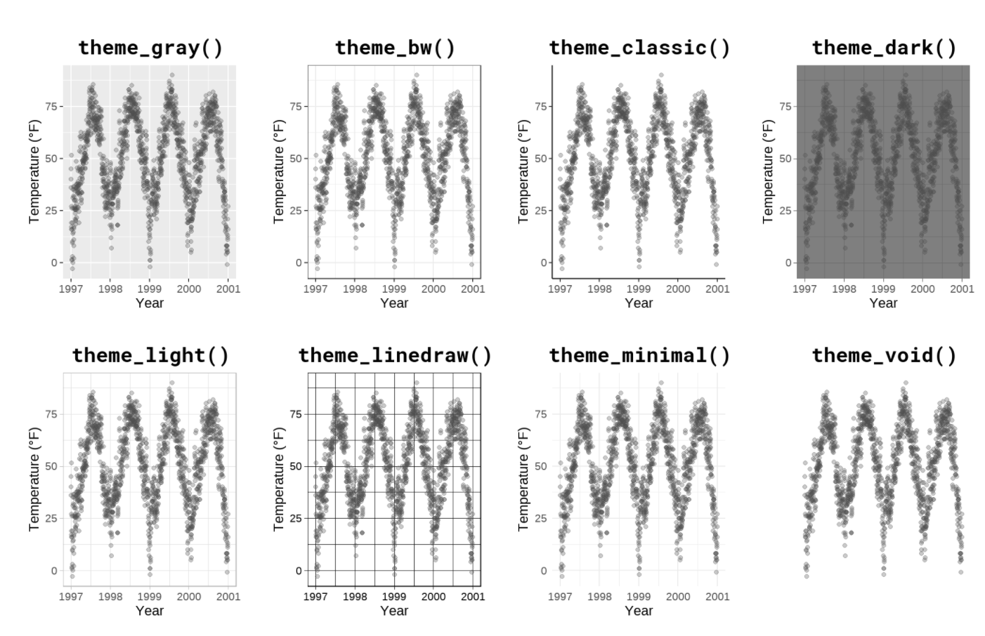
使用ggthemes这个包，还可以有很多主题可以选。

https://github.com/jrnold/ggthemes

https://github.com/BTJ01/ggthemes/tree/master/inst/examples

library(ggthemes)

ggplot(chic, aes(x = date, y = temp, color = season)) + geom_point() + labs(x = "Year", y = "Temperature (°F)") + ggtitle("Ups and Downs of Chicago's Daily Temperatures") + theme_fivethirtyeight() + theme(title = element_text(size=7))+ scale_color_economist(name = NULL)

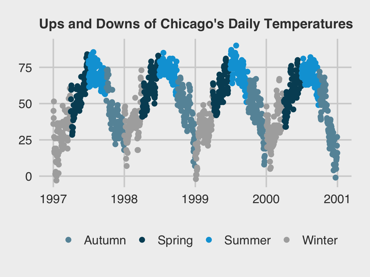
这是美国538网站的配色。

还有耶鲁Edward Tufte（them——tufte）教授的简明突出的风格也非常受人追捧。（此处参考网友dandelion资料）https://www.edwardtufte.com/tufte/books_vdqi

http://motioninsocial.com/tufte/

反正你看多了，就觉得是那种老式教科书的印刷风。还蛮有特色的。

其他推荐的包括ggsci,hrbrthemes。

这期内容太短了。再补一点如何添加辅助线。

g <- ggplot(chic, aes(x = temp, y = dewpoint)) + geom_point(color = "dodgerblue", alpha = .5) + labs(x = "Temperature (°F)", y = "Dewpoint") g + geom_vline(aes(xintercept = median(temp)), size = 1.5, color = "firebrick", linetype = "dashed") + geom_hline(aes(yintercept = median(dewpoint)), size = 1.5, color = "firebrick", linetype = "dashed")

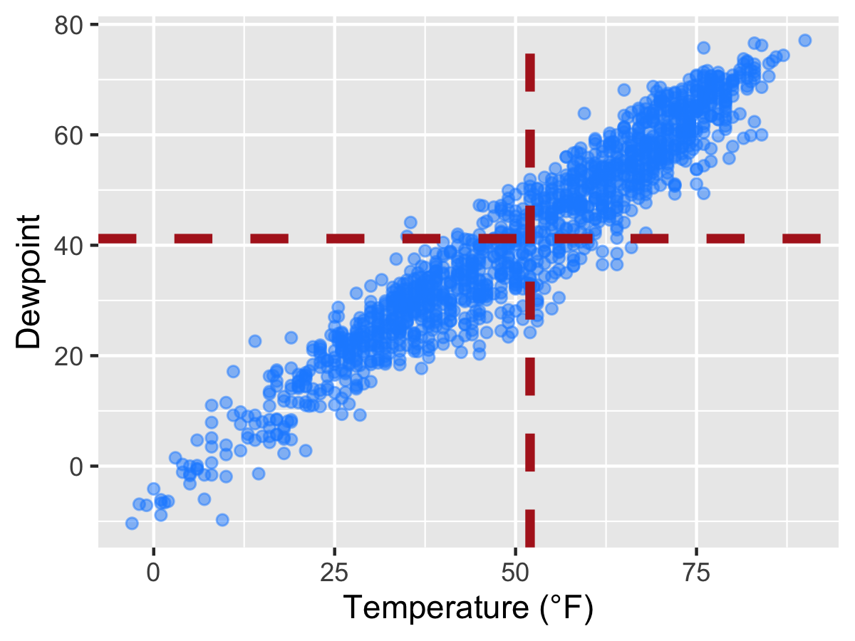
这里的vline是加垂直辅助线，hline是水平辅助线。后面可以用简单计算。

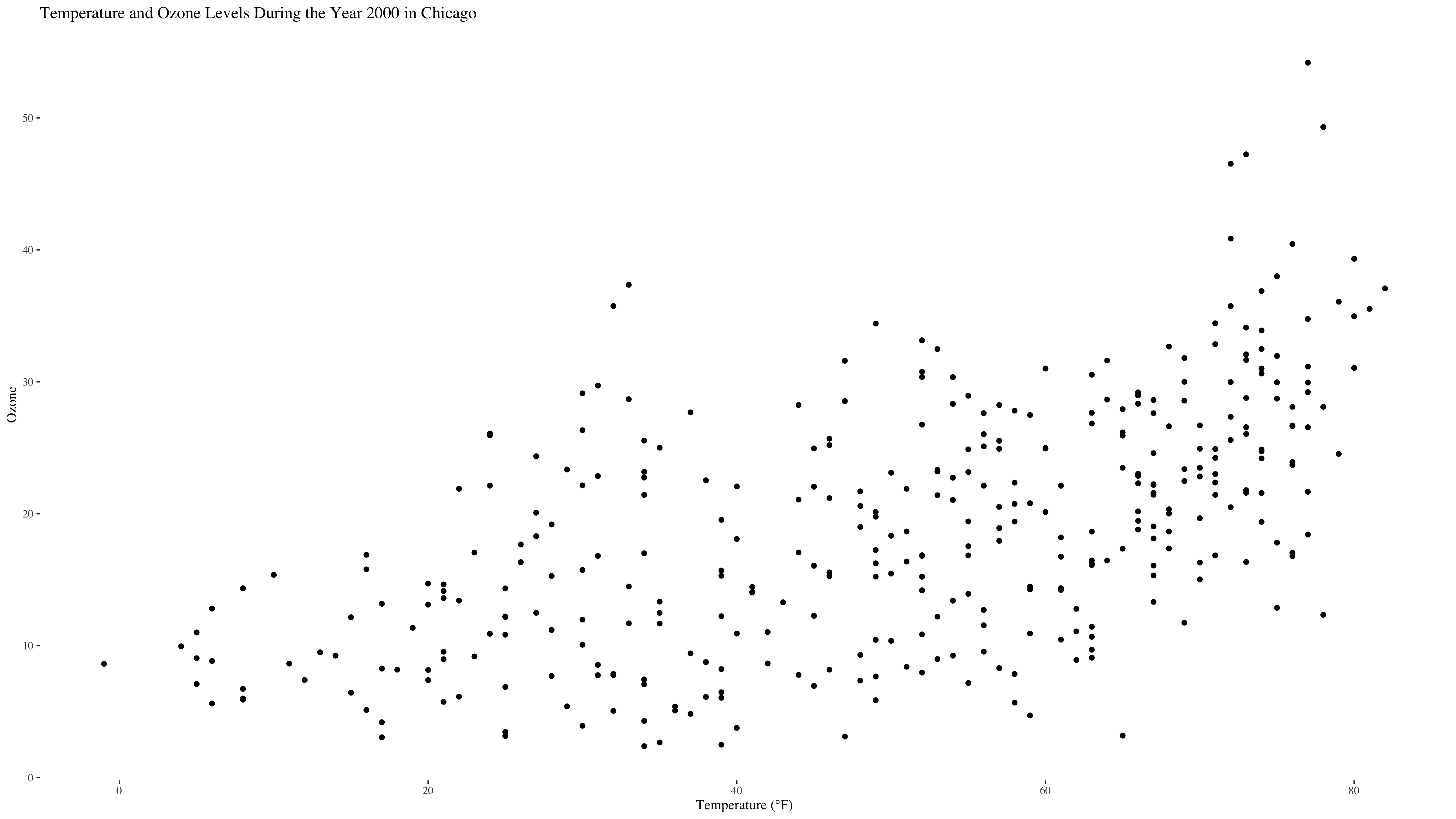
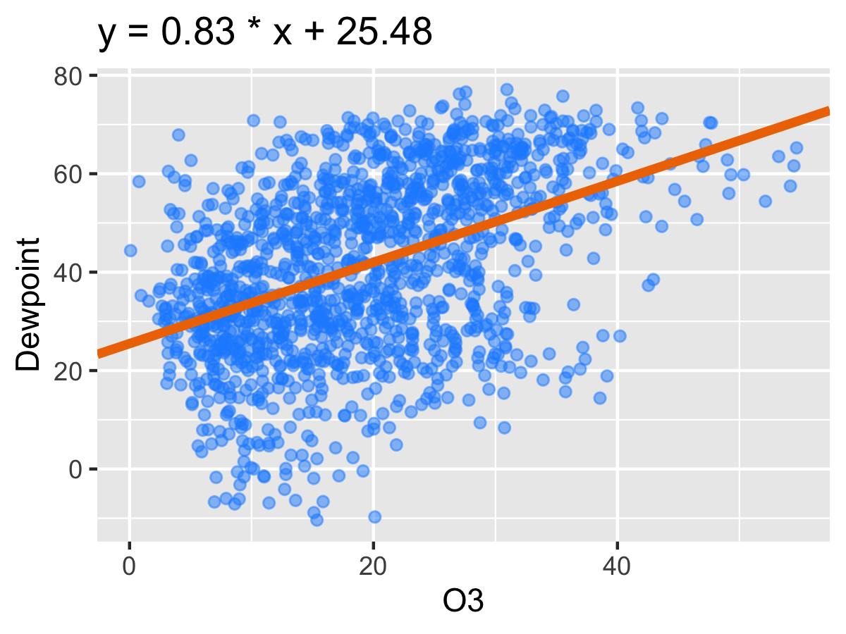
还可以加线性回归线。

g <- ggplot(chic, aes(x = o3, y = dewpoint)) + geom_point(color = "dodgerblue", alpha = .5) + labs(x = "O3", y = "Dewpoint")
reg <- lm(dewpoint ~ o3, data = chic)
g + geom_abline(intercept = coefficients(reg)[1], slope = coefficients(reg)[2],color = "darkorange2", size = 1.5) + labs(title = paste0("y = ", round(coefficients(reg)[2], 2), " * x + ", round(coefficients(reg)[1], 2)))

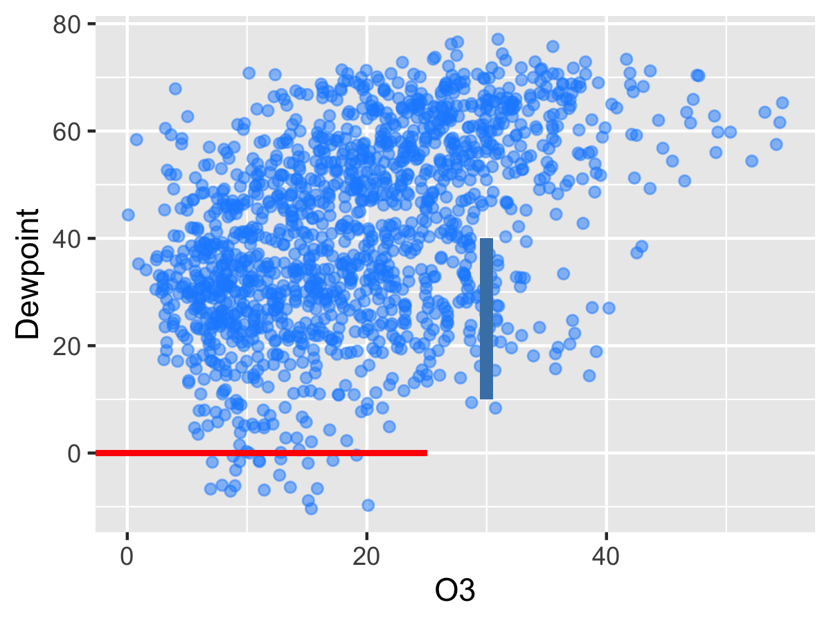
通过简单设置还可以加部分的线段，这个比较简单。就不细说了。

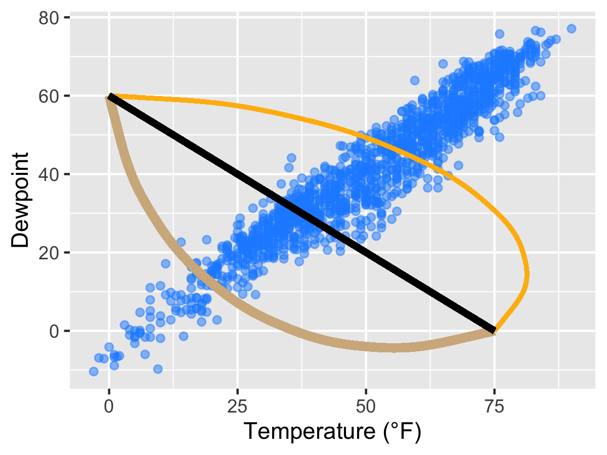
最后讲一下怎么做曲线出来。

g <- ggplot(chic, aes(x = temp, y = dewpoint)) + geom_point(color = "dodgerblue", alpha = .5) + labs(x = "Temperature (°F)", y = "Dewpoint")

p <- g + geom_curve(aes(x = 0, y = 60, xend = 75, yend = 0), size = 2, color = "tan") + geom_curve(aes(x = 0, y = 60, xend = 75, yend = 0), curvature = -0.7, angle = 45, color = "darkgoldenrod1", size = 1) + geom_curve(aes(x = 0, y = 60, xend = 75, yend = 0), curvature = 0, size = 1.5)

p <- g + geom_curve(aes(x = 0, y = 60, xend = 75, yend = 0), size = 2, color = "tan", arrow = arrow(length = unit(0.07, "npc"))) + geom_curve(aes(x = 0, y = 60, xend = 70, yend = 5), curvature = -0.7, angle = 45, color = "darkgoldenrod1", size = 1, arrow = arrow(length = unit(0.03, "npc"), type = "closed", ends = "both"))