@agpwhy 2022-01-11T14:42:14.000000Z 字数 5823 阅读 316

王胖的生信笔记第三十三期：河流图

前段时间小老板看到一个这样的图

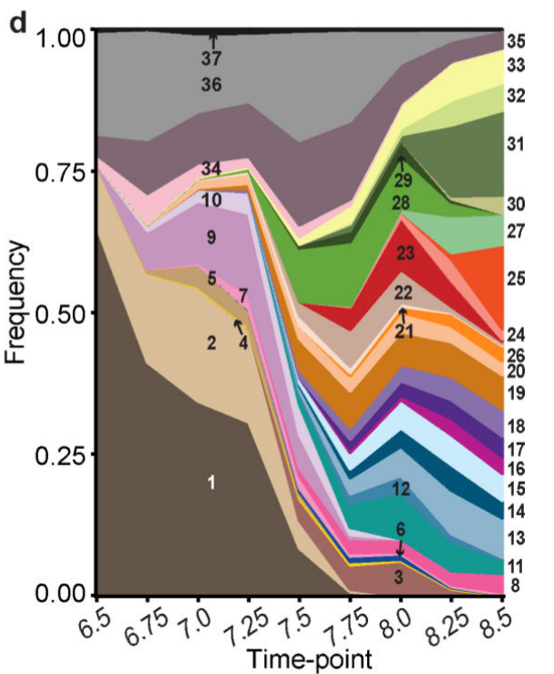
Donc让我去看下这个咋做。

首先不考虑直接用ggplot2去做（除非实在没有包）。于是问了一圈，有人和我说这个叫河流图（Stream Chart）。实际就是堆叠柱状图（Stack Bar Chart）的一个变种。

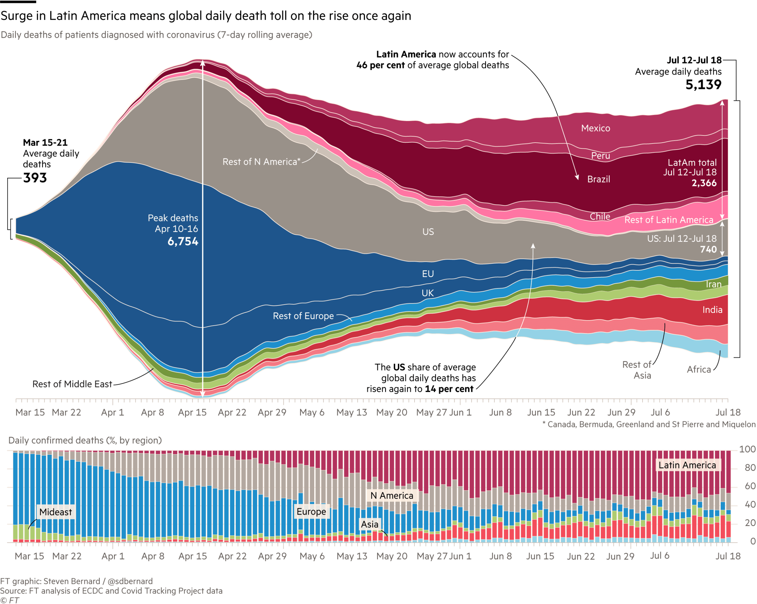
这样一看就明白了是啥意思了。

这自己咋整呢？

这里简单展示一下从TidyTuesday看到的一个示范。

配置环境

# https://github.com/z3tt/TidyTuesday/blob/master/R/2020_27_ClaremontRunXMen.Rmd
remotes::install_github("davidsjoberg/ggstream")
library(tidyverse)
library(fuzzyjoin)
library(ggstream)
library(colorspace)
library(ggtext)
library(ragg)
library(cowplot)
library(pdftools)

然后设置一下作图细节

theme_set(theme_minimal(base_family = "Helvetica", base_size = 12))
theme_update(
  plot.title = element_text(size = 27,
                            face = "bold",
                            hjust = .5,
                            margin = margin(10, 0, 30, 0)),
  plot.caption = element_text(size = 9,
                              color = "grey40",
                              hjust = .5,
                              margin = margin(20, 0, 5, 0)),
  axis.text.y = element_blank(),
  axis.title = element_blank(),
  plot.background = element_rect(fill = "grey88", color = NA),
  panel.background = element_rect(fill = NA, color = NA),
  panel.grid = element_blank(),
  panel.spacing.y = unit(0, "lines"),
  strip.text.y = element_blank(),
  legend.position = "bottom",
  legend.text = element_text(size = 9, color = "grey40"),
  legend.box.margin = margin(t = 30), 
  legend.background = element_rect(color = "grey40", 
                                   size = .3, 
                                   fill = "grey95"),
  legend.key.height = unit(.25, "lines"),
  legend.key.width = unit(2.5, "lines"),
  plot.margin = margin(rep(20, 4))
)

这里因为我电脑字体库的问题，所以用的是最简单的字体。

然后读取一下数据，修整清洗一下。

df_char_vis <- readr::read_csv('https://raw.githubusercontent.com/rfordatascience/tidytuesday/master/data/2020/2020-06-30/character_visualization.csv')
df_best_chars <-
  tibble(
    rank = 1:10,
    char_popular = c("Wolverine", "Magneto", 
                     "Nightcrawler", "Gambit",
                     "Storm", "Colossus",
                     "Phoenix", "Professor X",
                     "Iceman", "Rogue")
  )

这是关于X-men漫画系列的数据。里面有写名字大家熟悉，有些不行。Wolverine-金刚狼，Magneto-万磁王个，Nightcrawler-夜行者，Gambit-金牌手，Storm-暴风女，Colossus-钢力士，Phoenix-凤凰，Professor X-教授，Iceman-冰人，Rogue-罗刹女。

df_best_stream <-
  df_char_vis %>% 
  regex_inner_join(df_best_chars, by = c(character = "char_popular")) %>% 
  group_by(character, char_popular, costume, rank, issue) %>% 
  summarize_if(is.numeric, sum, na.rm = TRUE) %>% 
  ungroup() %>% 
  filter(rank <= 5) %>%
  filter(issue < 281)
#这里是整理数据类型，只展示那十位角色相关数据
df_smooth <-
  df_best_stream %>% 
  group_by(character, char_popular, costume, rank) %>% 
  slice(1:4) %>% 
  mutate(
    issue = c(
      min(df_best_stream$issue) - 20, 
      min(df_best_stream$issue) - 5,
      max(df_best_stream$issue) + 5,
      max(df_best_stream$issue) + 20
    ), 
    speech = c(0, .001, .001, 0), 
    thought = c(0, .001, .001, 0), 
    narrative = c(0, .001, .001, 0), 
    depicted = c(0, .001, .001, 0)
  )
levels <- c("depicted", "speech", "thought", "narrative")
df_best_stream_fct <-
  df_best_stream %>% 
  bind_rows(df_smooth) %>% 
  mutate(
    costume = if_else(costume == "Costume", "costumed", "casual"),
    char_costume = if_else(
      char_popular == "Storm",
      glue::glue("{char_popular} ({costume})"),
      glue::glue("{char_popular} ({costume})   ")
    ),
    char_costume = fct_reorder(char_costume, rank)
  ) %>% 
  pivot_longer(
    cols = speech:depicted,
    names_to = "parameter",
    values_to = "value"
  ) %>% 
  mutate(parameter = factor(parameter, levels = levels))

准备作图

这里是准备配色

pal <- c(
  "#FFB400", lighten("#FFB400", .25, space = "HLS"),
  "#C20008", lighten("#C20008", .2, space = "HLS"),
  "#13AFEF", lighten("#13AFEF", .25, space = "HLS"),
  "#8E038E", lighten("#8E038E", .2, space = "HLS"),
  "#595A52", lighten("#595A52", .15, space = "HLS")
)
labels <- 
  tibble(
    issue = 78,
    value = c(-21, -19, -14, -11),
    parameter = factor(levels, levels = levels),
    label = c("Depicted", "Speech\nBubbles", "Thought\nBubbles", "Narrative\nStatements")
  )
texts <-
  tibble(
    issue = c(295, 80, 245, 127, 196),
    value = c(-35, 35, 30, 57, 55),
    parameter = c("depicted", "depicted", "thought", "speech", "speech"),
    text = c(
      '**Gambit** was introduced for the first time in issue #266 called "Gambit: Out of the Frying Pan"— nevertheless, he is the **4<sup>th</sup> most popular X-Men character**!',
      '**Wolverine is the most popular X-Men** and has a regular presence in the X-Men comics between 1975 and 1991.',
      '**Storm** is by far the most thoughtful of the five most popular X-Men characters, especially in issues #220, #223 and #265. Storm **ranks 5<sup>th</sup>**.',
      "**Magneto** was ranked by IGN as the *Greatest Comic Book Villain of All Time*. And even though he only appears from time to time he **ranks 2<sup>nd</sup>**—<br>4 ranks higher than his friend and opponent Professor X!",
      'The **3<sup>rd</sup> most popular X-men character Nightcrawler** gets injured during the "Mutant Massacre"  and fell into a coma after an attack from Riptide in issue #211.'
    ),
    char_popular = c("Gambit", "Wolverine", "Storm", "Magneto", "Nightcrawler"),
    costume = "costumed",
    vjust = c(.5, .5, .4, .36, .38)
  ) %>% 
  mutate(
    parameter = factor(parameter, levels = levels),
    char_costume = if_else(
      char_popular == "Storm",
      glue::glue("{char_popular} ({costume})"),
      glue::glue("{char_popular} ({costume})   ")
    ),
    char_costume = factor(char_costume, levels = levels(df_best_stream_fct$char_costume))
  )

最后就作图

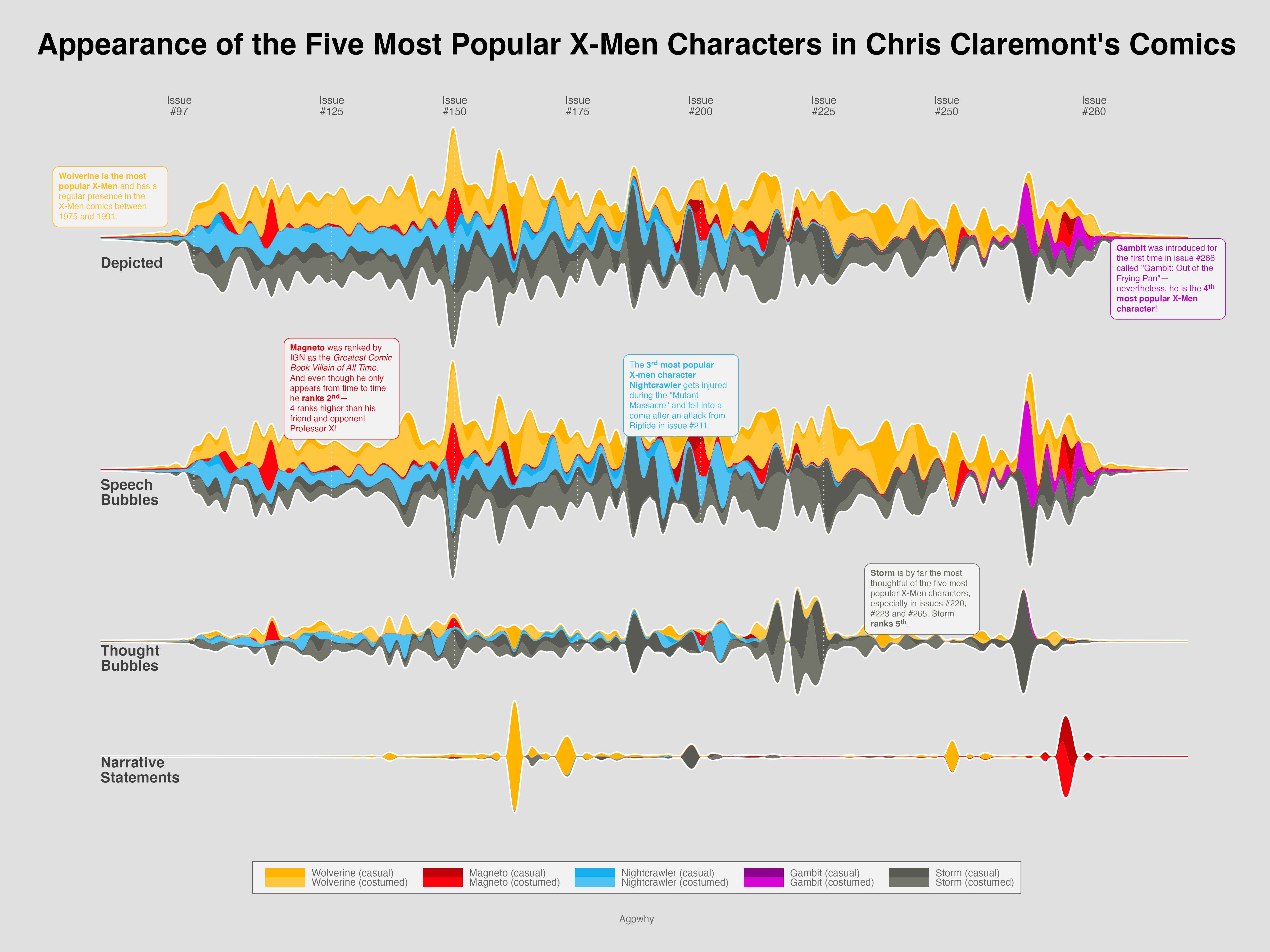
g <- 
  df_best_stream_fct %>% 
  ggplot(aes(
    issue, value, 
    color = char_costume, 
    fill = char_costume
  )) +
  geom_stream(
    geom = "contour",
    color = "white",
    size = 1.25,
    bw = .1
  ) +
  geom_hline(yintercept = 0, color = "grey88") +
  geom_stream(
    geom = "polygon",
    #n_grid = 12000,
    bw = .1,
    size = 0
  ) +
  geom_vline(
    data = tibble(x = c(97, seq(125, 250, by = 25), 280)),
    aes(xintercept = x),
    inherit.aes = F, 
    color = "grey88", 
    size = .5,
    linetype = "dotted"
  ) +
  annotate(
    "rect",
    xmin = -Inf, xmax = 78, 
    ymin = -Inf, ymax = Inf,
    fill = "grey88"
  ) +
  annotate(
    "rect",
    xmin = 299, xmax = Inf, 
    ymin = -Inf, ymax = Inf,
    fill = "grey88"
  ) +
  geom_text(
    data = labels,
    aes(issue, value, label = label),
    inherit.aes = F,
    family = "Helvetica",
    size = 4.7,
    color = "grey25",
    fontface = "bold",
    lineheight = .85,
    hjust = 0
  ) +
  facet_grid( ## needs facet_grid for space argument
    parameter ~ ., 
    scales = "free_y", 
    space = "free"
  ) +
  scale_x_continuous(
    limits = c(74, NA),
    breaks = c(94, seq(125, 250, by = 25), 280),
    labels = glue::glue("Issue\n#{c(97, seq(125, 250, by = 25), 280)}"),
    position = "top"
  ) + 
  scale_y_continuous(expand = c(.03, .03)) + 
  scale_color_manual(
    expand = c(0, 0),
    values = pal,
    guide = F
  ) +
  scale_fill_manual(
    values = pal,
    name = NULL
  ) +
  coord_cartesian(clip = "off") +
  labs(
    title = "Appearance of the Five Most Popular X-Men Characters in Chris Claremont's Comics",
    caption = "Visualization by Cédric Scherer  •  Data by Claremont Run Project via Malcom Barret  •  Popularity Scores by ranker.com  •  Logo by Comicraft"
  ) 
g <- g+theme(title = element_text(vjust = .5, hjust = .5))

2020_27_Xmen_clean

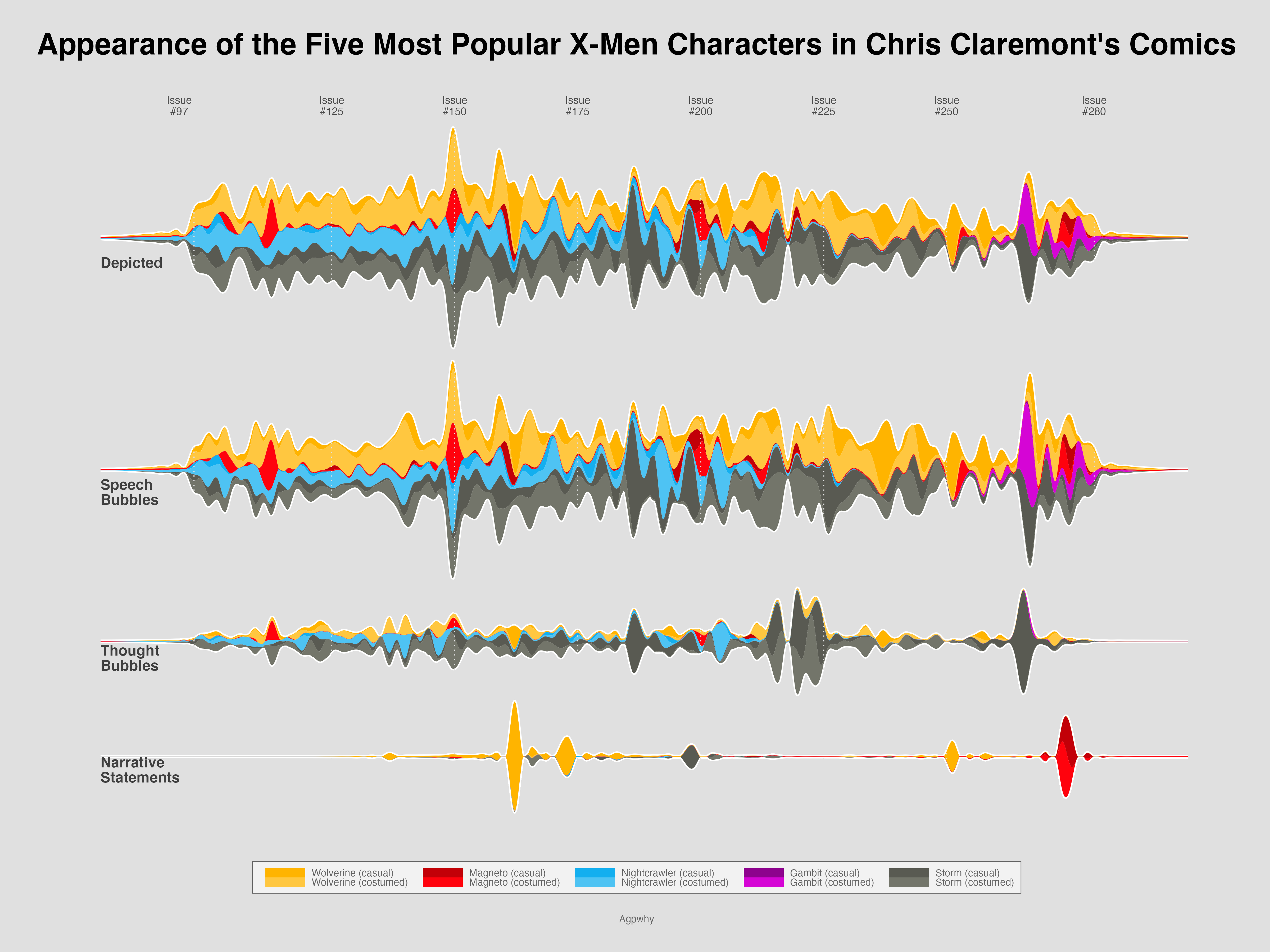
通过这样的可视化，可以看到金刚狼从所有统计的时间段（1975-1991）都非常有人气；万磁王人气排名第二；夜行者也是人气角色；暴风女虽然人气不如其他几人，但是在漫画中的思想描述最多；金牌手一直到266册才首次登场，但马上就有了大量存在感。

王胖的生信笔记第三十三期：河流图

配置环境

准备作图

内容目录